Suppose we observe a handful of points and want to predict the target at an input we have not seen. Drawing a curve through the observations is easy; deciding what that curve means is harder. Why should we prefer one curve over another? How much should we trust its prediction? If several curves explain the data nearly equally well, what happens to the alternatives we did not choose?
We will approach these questions through polynomial curve fitting, following the example in Bishop’s Pattern Recognition and Machine Learning
The mathematics will become richer, but the model will change very little. When the same curve-fitting problem is viewed from several angles, we can see exactly what each new assumption buys us.
Important
You do not need to memorize every symbol as it appears. The notation table is there when a symbol has slipped your mind.
1. One curve from least squares
Let
be a dataset of input-target pairs. Our immediate task is to construct a function that predicts the target corresponding to a new input .
For now, the inputs are treated as fixed. We are not claiming that inputs are never random; we are choosing to condition on the values we observed. This fixed-design viewpoint lets us focus on uncertainty in the targets and, later, in the model parameters without worrying about the inputs.
1.1 A model that is linear in its parameters
Assume first that an th-degree polynomial is flexible enough to represent the pattern of our dataset:
where:
is the parameter vector. When , the function is nonlinear in the input , but it is still linear in the parameters: each appears only to the first power, multiplied by a known function of . It is this second kind of linearity that makes the model a linear regression model.
Polynomial notation is familiar, but it hides a useful general pattern. This is where linear algebra comes in. Let and define the basis functions:
Collecting them gives us the feature vector:
so the polynomial can be written as a dot product:
Nothing in this form requires monomials. We could replace the components of —the monomials in this case—with splines, Fourier functions, radial basis functions, or another fixed collection of features. Once has been chosen, the model remains linear in . The feature map determines which shapes the model can express; the parameters determine which of those shapes it selects
1.2 Seeing all observations at once
Evaluating the feature vector at every training input produces the design matrix:
Similarly, collect the observed targets into:
For any proposed parameter vector , the product:
contains the model’s predictions at all training inputs.
1.3 How to choose one best-fitting curve
We know that the model is a polynomial parameterized by . The next question is: how do we choose the best-fitting curve for our data? We need a way to measure the discrepancy between the model predictions and the observed targets.
The larger the discrepancy, the worse the fit. We measure this discrepancy with a loss function, then seek the parameter vector that minimizes it.
For a parameter vector , we define the residual vector as:
We define the loss function as the sum of squared residualsThe factor does not change which parameters minimize the objective; it merely cancels the factor that appears when we differentiate a square.:
A least-squares estimate is any parameter vector satisfyingWe write rather than because the minimizing parameter vector need not be unique. If the columns of are linearly dependent, different parameter vectors can produce identical predictions at every training input.:
1.4 Solving for the fitted curve
To find a least-squares estimate, differentiate the objective:
Setting the gradient to zero gives the normal equations:
The normal equations also have a geometric meaning. Rewrite them as
Every attainable vector of fitted training values lies in the column space . The equation says that the fitted residual is orthogonal to every column of , and therefore to that entire model space. Thus is the closest point in the model space to .
The next figure shows the exact geometry when the observation space is two-dimensional and the model space is a line. Moving along the line changes both the residual length on the left and the squared loss on the right; the orthogonal projection and the bottom of the loss curve identify the same fit
The closest prediction is the bottom of the loss
Drag the gold candidate in either view
The Hessian is , and for every :
Therefore is convex, so every solution of the normal equations is a global minimizer. If has full column rank, the Hessian is positive definite, the minimizer is unique, and:
If is rank deficient, a minimizer still exists and the fitted training vector is unique, but multiple parameter vectors can represent it. The inverse formula is then unavailableEven when the inverse exists, explicitly forming it is usually a poor numerical method. Practical least-squares solvers use QR or singular-value decompositions because the normal equations can worsen conditioning
At this stage, squared error is a choice, not a consequence. It says that positive and negative residuals of the same magnitude are equally costly, and that a residual twice as large contributes four times as much. Those properties may be reasonable, but least squares alone does not tell us why they should describe the data.
This leaves a more basic question: what would it mean for one parameter vector—or one curve—to be more plausible than another?
2. A bridge into the Bayesian world
Least squares gives us an optimization problem. Bayesian inference will give us a language for uncertainty. Before connecting the two, we need to distinguish three objects that are often collapsed in informal explanations: a discrepancy, a probability model for the observations, and uncertainty about the parameters themselves.
The distinction matters because a small training error does not imply that the fitted curve is known with certainty. With limited data, many curves may remain plausible even when an optimizer returns only one of them. Bayesian machine learning begins by refusing to silently discard those alternatives.
2.1 What becomes uncertain?
In least squares, is an unknown but fixed parameter. We search through and retain a value that minimizes . The hat in reminds us that this value was estimated from data, but the estimate itself is still a single point.
Bayesian inference represents our uncertainty about with a probability distribution. Imagine that the curve has one fixed but unknown parameter vector. Before seeing the data, many values of may be plausible. After seeing the data, values that produce curves inconsistent with the observations become less plausible. The data change our distribution over ; they do not cause the parameter itself to move or be redrawn.
This is separate from noisy observations. Even if were known exactly, repeated targets at the same input could still differ. Conversely, the observations could be almost noiseless while limited data leave several parameter values plausible. Bayesian prediction will eventually account for both sources, but they enter through different parts of the model.
2.2 Bayes’ theorem as an update rule
Let denote the observed dataset and, for the moment, suppress the fixed training inputs from the notation. The product rule gives two ways to factor the same joint distribution:
Equating the two factorizations and dividing by gives Bayes’ theorem:
Each term has a different role:
- The prior describes our uncertainty about the parameters before using .
- The likelihood measures how compatible the observed data are with each proposed parameter value.
- The posterior describes our updated uncertainty after using the data.
- The evidence is the probability or density assigned to the observed data by the model as a whole.
For a continuous parameter vector , the evidence is obtained by averaging the likelihood under the prior. This is also known as marginalization:
Provided , the evidence normalizes the numerator so that the posterior integrates to one. It does not depend on the particular value of under consideration, so we can treat it as a constant with respect to . We may therefore describe the shape of the posterior by writing:
2.3 What is the likelihood?
The expression can be read in two related ways. If is fixed and possible datasets vary, it is a probability mass function or density over the data. Once has been observed, we hold it fixed and view the same expression as a function of :
This function is the likelihood. The semicolon is a reminder that varies while the observed dataset is fixed.
Likelihood is not, by itself, a probability distribution over . In general:
need not equal one. The likelihood can rank parameter values by how well they explain the same observations, but a prior and the evidence are needed to turn those relative weights into a posterior distribution.
This gives us the first connection to ordinary model fitting. Maximum-likelihood estimation (MLE) retains the parameter value at the peak of the likelihood:
It uses a probability model for the observations, but its output is still one parameter estimate.
2.4 From MLE to MAP and beyond
Once a prior has been specified, we could instead retain the parameter value at the peak of the posterior. This is the maximum a posteriori, or MAP, estimate:
The evidence disappears from the optimization because it is constant with respect to . MAP does not maximize the likelihood and prior separately; it chooses the mode of their product.
If the prior density is constant over all parameter values relevant to the optimization, then it does not change their ranking. In that case:
whenever the corresponding optimizer is uniqueA proper uniform distribution over all of does not exist. A “flat prior” may instead mean a proper prior that is constant on a bounded admissible region, or an improper constant density used as a formal device. In the latter case, we must still check that the resulting posterior is proper..
But MAP is not the final destination of Bayesian inference. It uses the posterior and then collapses it back to one point. If two separated regions of parameter space are both plausible, their relative mass is lost once we report only the highest point.
Full Bayesian inference retains the posterior distribution. For prediction at a new input , it averages the prediction associated with every possible parameter value, weighted by posterior plausibility:
After integrating over , the predictive distribution no longer conditions on one chosen parameter value. A sharply concentrated posterior may make this average resemble prediction with a single estimate. A broad or multimodal posterior can make the difference substantial.
Summary (Three procedures, three retained objects)
- MLE uses the likelihood and retains one parameter estimate.
- MAP uses the posterior and retains one parameter estimate.
- Full Bayesian inference retains parameter uncertainty and averages over it when making predictions.
We now have the roadmap, but one part is still abstract: the likelihood. What probability model for the targets would make smaller squared residuals more plausible, and would recover our least-squares objective through maximum likelihood? Gaussian observation noise gives an exact answer.
3. Gaussian noise turns least squares into likelihood
Least squares began with a loss function. It compared the fitted curve with the targets we happened to observe, but it said nothing about which other targets we might have observed instead. A likelihood requires that missing piece: a probability model for the targets.
We are still one step short of Bayesian linear regression. In this section, probability enters through the observations, while and the noise level remain fixed but unknown parameters. We will estimate them rather than place distributions over them.
3.1 A stochastic model for the targets
Keep the training inputs fixed. For each input, suppose the corresponding target can be approximated by our linear model, but life is not perfect: there is always some mismatch between the model and the target.
This mismatch or error is represented by a random noise variable :
The parameter is called the noise precision. Precision is the reciprocal of variance, so a larger means that observations are more tightly concentrated around the curve We usually use and for a “standard” notation when a random variable has a normal distribution. But here, we use , or the precision, instead. The goal is to make the derivation more convenient and also more consistent with Bayesian literature.:
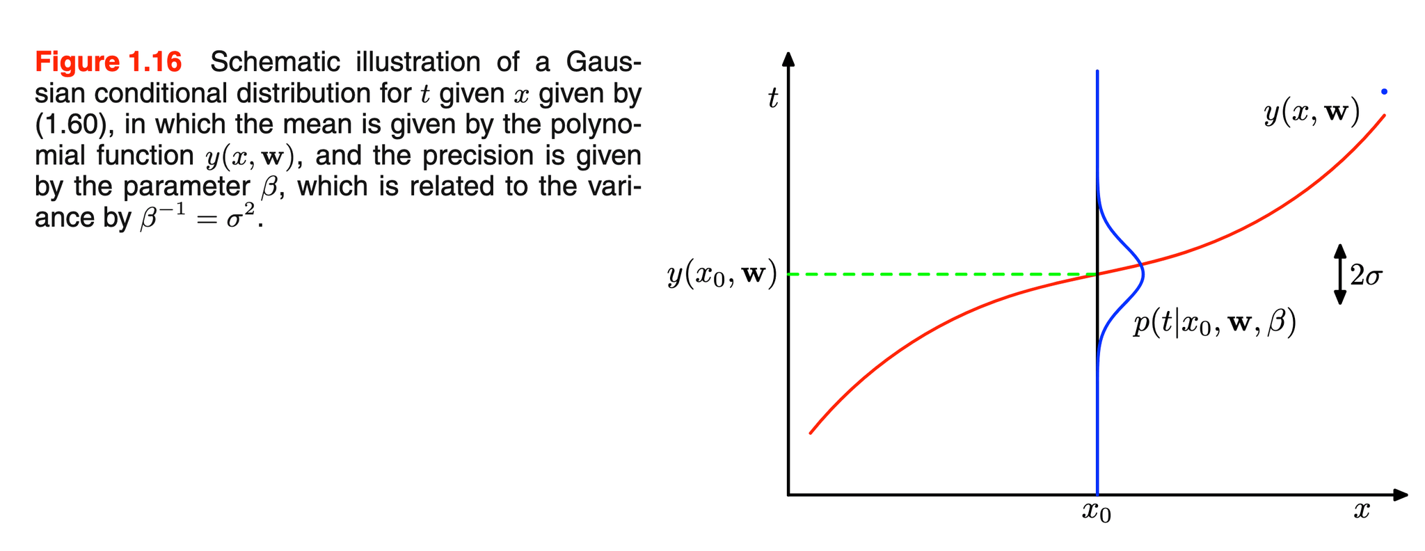
The curve with a Gaussian noise model from Bishop
Equivalently, the conditional distribution of each target is:
The curve now has a probabilistic meaning: it is the conditional mean of the target.
Zero-mean noise does not say that every observed residual must be zero. It says that if we repeatedly generated a target at the same input while holding and fixed, the residuals would average to zero under the model.
Collect the random targets into . The scalar assumptions can then be written as one multivariate Gaussian:
The covariance matrix records two assumptions: every target has the same conditional variance, and the observation errors are independent once the inputs and parameters are fixedThe targets themselves are not identically distributed when their inputs give different means. The centered errors are i.i.d..
Caveat (Gaussian noise is an assumption).The Gaussian model is not forced upon us by least squares. It can be a poor description of outliers, asymmetric errors, bounded targets, counts, or noise whose variance changes with the input. Different observation models produce different likelihoods and usually different losses.
3.2 From the observation model to a likelihood
We have observed the numerical target vector . Because the targets are conditionally independent, their joint density is the product of the individual Gaussian densities:
Holding and fixed while varying and turns this density into the likelihood:
Substituting the Gaussian density gives:
where the observed quantities have been suppressed from the notation. The residual norm from least squares has reappeared, now inside a probability density.
Products of many densities are inconvenient to manipulate and can become numerically tiny. Since the logarithm is strictly increasing, maximizing the likelihood is equivalent to maximizing the log-likelihood:
Using the least-squares loss , the same expression becomes:
Drag one residual through probability and loss
The negative logarithm reverses the ranking without moving the optimum
This identity is the bridge back to our original optimization problem. The figure isolates one residual, but conditional independence makes the dataset log-likelihood a sum of terms with the same shape
3.3 Maximum likelihood recovers least squares
Fix any noise precision . The first two terms of do not depend on , and the coefficient of is strictly negative. Therefore:
The maximizing set is the same for every fixed . Consequently, whenever a finite joint maximum over exists, its component is a least-squares estimate. Conversely, any least-squares estimate maximizes the likelihood over when is fixed:
We can now answer why squared error appeared: under independent Gaussian observation noise with constant variance, the negative log-likelihood differs from a positive multiple of squared error only by terms that do not depend on
This is an equivalence between two optimization problems under stated assumptions. It does not prove that Gaussian noise is correct for a particular dataset. Rather, it tells us exactly which probability model makes least squares a maximum-likelihood procedure.
The least-squares solution from Section 1 is therefore also the maximum-likelihood solution for under this observation model. The curve has not changed; only our interpretation of its objective has.
3.4 Estimating the noise precision
The parameter vector determines the center of the Gaussian observation model. Its precision determines how tightly possible targets cluster around that center. We can estimate it from the same likelihood.
Let:
be the residual sum of squares at a least-squares solution, which also maximizes the likelihood over for every fixed . Every such solution produces the same fitted training vector, so is well defined even if the parameter vector is not unique.
With fixed, the log-likelihood becomes:
Assume first that . Differentiating with respect to gives:
Setting this derivative to zero yields:
The second derivative is
so this stationary point is the unique maximum over .
Caveat (An exact fit has no finite precision estimate).If , the fitted curve interpolates every training target. The log-likelihood then increases without bound as , or equivalently as the noise variance approaches zero. In this case, no finite maximum-likelihood estimate of exists, and the formula must not be used.
3.5 Prediction after maximum likelihood
For a new fixed input , the same observation model says:
Substituting the maximum-likelihood estimates gives the plug-in predictive distribution:
The mean is our familiar curve evaluated at the new input:
The variance describes how a new observation can vary around that curve according to the fitted noise model. It does not express uncertainty about the estimated parameters themselves.
3.6 The uncertainty that maximum likelihood discards
The plug-in distribution looks probabilistic, but it treats and as if the data had revealed their exact values. It therefore handles one source of uncertainty while discarding another:
- Observation uncertainty: even if the parameters were known, a new target could differ from the curve because of . The plug-in distribution retains this variation.
- Parameter uncertainty: finite data can leave many values of plausible. Substituting discards this uncertainty.
The difference becomes visible when we extrapolate. Under the constant-variance Gaussian model, the plug-in distribution has the same width at every input. It is just as narrow far away from the training data as it is near them, even though the fitted curve is usually much less constrained there.
This is the limitation that motivates the next step. We will place a prior distribution over , update it with the Gaussian likelihood, and carry the resulting posterior uncertainty into prediction.
4. A Gaussian prior and the MAP estimate
Maximum likelihood asks which parameter value makes the observations most plausible. It has no way to express which parameter values seemed plausible before seeing those observations. A prior supplies that missing information.
To keep the next derivation focused, we will treat the noise precision as fixed and introduce uncertainty only over . We will also introduce a second precision parameter, , that controls the prior. Both are hyperparameters: they determine the shapes of distributions over other quantities rather than directly determining the fitted curveA more complete Bayesian model could place priors over and as well. Treating them as fixed lets us first see the central update for without another layer of integration..
4.1 A prior over the weights
Choose an isotropic zero-mean Gaussian prior:
Written as a density, this is:
The prior assigns its largest density to and gradually less density to parameter vectors with larger Euclidean norm. It does not assert that the weights are zero. It says, before using the targets, that smaller weights are more plausible than very large ones under this model.
The precision controls how strongly the prior concentrates around zero:
- A large gives a narrow prior and expresses a stronger preference for small weights.
- A small gives a broad prior and allows a wider range of weights.
This prior is convenient, but it is still an assumption. Zero mean treats positive and negative coefficients symmetrically, while the covariance treats every coefficient as independent and equally variable. Those choices may be unsuitable when features have very different meanings or scales.
4.2 Combining the prior and likelihood
Bayes’ theorem gives the posterior up to its normalizing evidence:
Substituting the Gaussian likelihood and prior gives:
The likelihood favors weights whose curve agrees with the observed targets. The prior favors weights close to zero. The posterior combines both preferences rather than choosing between them.
Move the evidence, watch the posterior negotiate
Posterior ∝ likelihood × prior; precision determines the pull
The figure shows the standard one-dimensional Gaussian conjugate update
4.3 The MAP objective
The MAP estimate is the mode of this posterior. Since the logarithm is strictly increasing, maximizing the posterior is equivalent to minimizing its negative logarithm. Terms that do not depend on can be dropped, leaving:
The first term rewards agreement with the data; the second penalizes large weights. Dividing the whole objective by does not change its minimizer, so we can also write:
This is the objective used by ridge regression, or -regularized least squares. From the optimization viewpoint, is a regularization strength. From the probabilistic viewpoint, it is the ratio between prior precision and observation precision.
4.4 Solving for the MAP estimate
Differentiating the MAP objective gives:
Setting this gradient to zero yields:
Because , the matrix is positive definite even when is rank deficient. The MAP estimate is therefore unique:
Equivalently,
As , the prior becomes flatter and the MAP objective approaches least squares. For positive , the prior pulls the solution toward zero and resolves parameter non-uniqueness by preferring the smaller-norm explanation.
MAP has improved the optimization problem, but its output remains one parameter vector. The posterior expression above contains more information than its mode. In the next step, we will identify the entire Gaussian posterior and see what uncertainty MAP leaves behind.
5. Keeping the whole posterior
The MAP estimate keeps only the highest point of the posterior. This is enough when our sole aim is to choose one parameter vector, but it cannot tell us whether that point is a sharp peak or merely the top of a broad hill. Those two posteriors have the same kind of summary—a mode—but express very different levels of certainty.
For our Gaussian likelihood and Gaussian prior, we do not need an approximation to recover the missing information. Their product is another Gaussian distribution, so the full posterior can be written exactly.
5.1 Recognizing the Gaussian
Return to the unnormalized posterior:
To identify this density, we need to rewrite its exponent as a quadratic centered at some vector. First expand the squared residual:
This notation defines
The matrix is positive definite because , so its inverse exists. We can therefore complete the square:
The last two terms do not depend on ; they become part of the normalizing constant. What remains has exactly the exponent of a multivariate Gaussian. Hence
This closed form is a consequence of conjugacy: the Gaussian prior and Gaussian likelihood combine to produce a posterior in the same distribution family as the prior. Conjugacy is not required for Bayesian inference, but here it lets us see every step without numerical integration
5.2 What the posterior mean remembers from MAP
The posterior mean is
This is exactly the MAP estimate derived in Section 4:
The equality is special to this Gaussian posterior. A Gaussian is symmetric around its mean, and its mean is also its unique mode. For a skewed or multimodal posterior, the posterior mean and MAP estimate can differ substantially.
The Bayesian update therefore does not discard the curve selected by MAP. It places that curve at the center of a distribution over alternative parameter vectors:
Each draw of from this posterior produces a different plausible curve . Parameter vectors close to in the geometry determined by receive more posterior density, while distant vectors receive less. MAP retains the center; full Bayesian inference retains the surrounding alternatives as well.
The next figure makes this correspondence visible in the special case . Then has only two components, so a point in weight space can be drawn on a page. That same point defines exactly one line in function space.
Drag a weight, watch the function move
The same w determines a location in posterior density and a line f(x, w)
This coupled view follows the weight-space constructions used by Bishop and by Rasmussen and Williams
5.3 Reading uncertainty from the covariance
The posterior covariance is
Its inverse has a particularly useful interpretation:
The update is additive in precision, not covariance. To make “direction” precise, choose any unit vector and restrict the posterior to a line . Its negative log-density has curvature
The prior contributes in every direction. The data contribute more curvature when moving along changes the fitted training values substantially. If , the likelihood is flat along that direction and contributes nothing; only the prior prevents the posterior from remaining flat.
The uncertainty of the scalar component is
These two directional quantities are exact, but they are not generally reciprocals: correlations can couple to other directions. They become reciprocals when is an eigenvector of . The useful conclusion survives without that shortcut—the likelihood constrains only parameter movements that change the model’s values at the observed inputs.
This also explains why the posterior remains well defined when the design matrix is rank deficient. Least squares cannot distinguish parameter vectors that differ in an unobserved direction. The Gaussian prior can: it supplies the positive precision even where the likelihood supplies none.
Important (Uncertain parameters do not always mean uncertain predictions)
Two parameter vectors can differ while producing nearly the same function over inputs we care about. Conversely, a modest amount of parameter uncertainty can become large predictive uncertainty at an input whose feature vector points in a poorly constrained direction. The covariance lives in parameter space; the feature vector will translate it into uncertainty about a prediction.
We now possess what MAP omitted: a distribution over the weights. The remaining step is to make a prediction without collapsing that distribution back to one fitted vector. We will do this by averaging the observation model over every parameter value in the posterior.
6. Prediction without collapsing the posterior
At a new input , maximum likelihood and MAP substitute one fitted weight vector into the observation model. Full Bayesian prediction takes a different route: it considers the prediction made by every possible and weighs that prediction by the posterior plausibility of .
The resulting posterior predictive distribution is
The integral is the essential Bayesian step. We do not have to decide which single is correct before predicting. Instead, parameter values with high posterior density contribute strongly, values with low posterior density contribute weakly, and the alternatives are averaged rather than discarded
6.1 From uncertain weights to an uncertain curve
Let
be the feature vector at the new input. Under the posterior,
The noise-free model value at is the scalar
A linear transformation of a Gaussian random vector is Gaussian. Therefore,
The mean is the curve obtained from the posterior mean , which is also the MAP estimate in our model. The variance is new. It measures how much the plausible curves disagree at the particular input .
Notice that this variance depends on the input through . The posterior over is the same no matter where we query it, but different inputs probe different directions in parameter space. Near well-supported inputs, the plausible curves may agree closely. Where the data constrain the curve poorly, they may spread apart.
6.2 Adding the uncertainty of a future observation
A future target is not just the noise-free curve value. The observation model also includes fresh noise:
The new noise is independent of the posterior uncertainty in . The sum of two independent Gaussian variables is Gaussian; their means and variances add. Thus the integral defining the posterior predictive distribution has the closed form
The predictive variance separates into two sources:
The first term is the irreducible variation assumed by our observation model. Even perfect knowledge of would not remove it. The second term records our incomplete knowledge of the curve. It can shrink as informative data constrain the weights, and it changes with the input.
This distinction also tells us which uncertainty to report:
- If we care about the latent mean function , its posterior variance is only .
- If we care about a future noisy target , its predictive variance also includes .
Calling both bands simply an “uncertainty interval” hides an important modeling choice. One describes uncertainty about the underlying curve; the other describes where a new observation may fall.
The distinction becomes easier to see if we inspect both distributions at the same input and then move that input through the domain.
Drag the question, separate the uncertainties
The latent curve and a future observation answer different questions
This linked construction follows the predictive-variance decomposition used in Bayesian linear regression
For example, under our Gaussian model,
is an approximate posterior credible interval for the latent value . It does not include the additional scatter of a future observation around that value.
6.3 What full Bayesian prediction adds
Compare the result with a plug-in prediction that substitutes the MAP estimate . The Bayesian and MAP plug-in predictive means agree:
The maximum-likelihood plug-in mean from Section 3 generally differs because need not equal . More importantly, either plug-in approach discards parameter uncertainty. A MAP plug-in distribution keeps only in its variance; Bayesian prediction also carries the posterior uncertainty in the weights:
This is why the Bayesian predictive band can widen away from the observations even though the assumed noise variance is constant. The noise has not increased; the plausible curves disagree more strongly there.
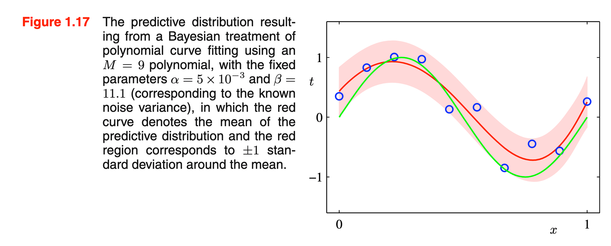
Bishop’s Bayesian polynomial curve fit. The red curve is the predictive mean and the shaded region extends one predictive standard deviation on either side
In the figure, the shaded region is narrower where the observations constrain the polynomial and wider near the boundaries, where many plausible weight vectors yield different curves. The width combines observation noise and parameter uncertainty; it should not be read as uncertainty in the red mean curve alone. The green curve is the function that generated Bishop’s synthetic data, shown for comparison. A real dataset would not reveal this ground-truth function to us.
For a Gaussian posterior predictive distribution, an interval
contains approximately of future targets under the model. This is a posterior predictive interval: unlike the plug-in predictive distribution in Section 3, it averages over uncertainty in . The statement is still conditional on our chosen feature map and on the fixed hyperparameters and .
The progression is now complete. Least squares chose one curve by minimizing error. A Gaussian noise model reinterpreted that choice as maximum likelihood. A Gaussian prior turned it into MAP and ridge regression. The full posterior retained the plausible alternatives, and the posterior predictive distribution carried their disagreement into the prediction.
Notation
The table below records the symbols that carry the main argument. We use , , and for random targets under the observation model; , , and denote realized values. Other uppercase symbols can have different roles: , for example, is a fixed matrix. A hat marks a fitted or estimated quantity.
| Symbol | Meaning | Shape or domain | Role |
|---|---|---|---|
| Training dataset | input-target pairs | Observed | |
| Input for observation | Fixed design | ||
| / | Observed target / target before observation | Observed / random | |
| Feature vector at input | Fixed transformation | ||
| Design matrix | Fixed after observing the inputs | ||
| Model parameters | Optimized first; uncertain later | ||
| / | Observed / random target vector | Observed / random | |
| Observation-noise precision | Estimated first; possibly uncertain later | ||
| Prior precision for | Fixed hyperparameter | ||
| MAP regularization strength | Derived hyperparameter | ||
| Posterior mean of | Inferred from the data | ||
| Posterior covariance of | Inferred uncertainty | ||
| New input | Fixed query | ||
| Latent noise-free model value at | Random under the posterior | ||
| / | Realized / random future target | Prediction |
References
- [Bishop, 2006]Pattern Recognition and Machine Learning[HTML]Bishop, Christopher M., 2006. Springer.
- [Trefethen et al., 1997]Numerical Linear Algebra[DOI]Trefethen, Lloyd N. and Bau, David, 1997. Society for Industrial and Applied Mathematics.
- [Rasmussen et al., 2006]Gaussian Processes for Machine Learning[HTML]Rasmussen, Carl Edward and Williams, Christopher K. I., 2006. MIT Press.
- [Murphy, 2022]Probabilistic Machine Learning: An Introduction[HTML]Murphy, Kevin P., 2022. MIT Press.
- [MacKay, 2003]Information Theory, Inference, and Learning Algorithms[HTML]MacKay, David J. C., 2003. Cambridge University Press.
- [Yu et al., n.d.]Bayesian Neural Networks[HTML]Yu, Jerry Qinghui, Creager, Elliot, Duvenaud, David, et al., n.d..