Danger
This article was originally written in Vietnamese. The following is an English translation with improvements created with the assistance of GPT 5.6 Sol to make the content accessible to a broader audience.
1. The Agent-Environment Interaction
Before writing down any equations, let’s agree on the picture we have in mind. Reinforcement Learning is still Machine Learning, but the data does not arrive as a fixed dataset as in Supervised Learning: the agent gathers it by interacting with the world, and its actions change what it will encounter next. We therefore need to think in terms of a continuous loop of action and feedback.
The two main components of Reinforcement Learning (RL) are the Agent and the Environment.
- The environment is the world that the agent lives in and interacts withThe Boundary Between Agent and Environment: This boundary is not physical (like the skin of a robot). Anything the Agent cannot change arbitrarily is considered part of the Environment (e.g., a robot’s battery level, as the Agent cannot command “Battery, become full” arbitrarily)..
- At each step (or time step), the agent perceives itself to be in a state of the environment and, based on that state, decides what it needs to doAccording to
[Achiam, 2018] , there are two definitions we need to distinguish: state (a complete description of the world, like chess) and observation (an incomplete description, like poker). In this context, we assume descriptions are always complete, so ..
After performing an action, the agent receives a scalar reward signal (or simply reward) associated with the resulting transition. A reward need not measure the quality of the current state by itself; it may depend on the preceding state, action, and next state. Usually, it is a real number and indicates how good or bad the action or the current state is.
The agent’s goal is to maximize the cumulative reward it receives over time. We call this accumulated reward the Return.
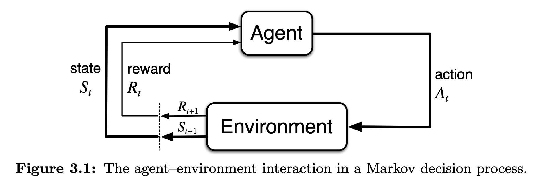
A Markov Decision Process (MDP) is a mathematical framework used to formalize sequential decision making problems. In this problem, at each time step, the agent must make a decision (action) based on the state. The agent’s action influences not just the immediate reward and next state, but also future rewards and states.
An MDP is appropriate when the chosen state representation contains the information needed to model future transitions and rewards. Within that model, interaction is summarized by three signals crossing the agent-environment boundary: the state on which a decision is based, the action selected by the agent, and the resulting reward.
The term
We can formalize this process as follows:
- At each time step , the agent receives a representation of the environment’s state, , where is the set of all possible states.
- Based on , the agent selects an Action (note that the set of available actions may differ per state).
- One time step later (at ), the agent receives a reward and finds itself in a new state .
This sequence of interactions forms a trajectory. Where do and come from? We sample from an initial-state distribution, and then the policy selects . This distribution matters because it changes which parts of the MDP we are likely to visit—and therefore which behavior our overall performance measure emphasizes (read more here).
In a finite MDP, the sets are all finite. Under the Markov and time-homogeneity assumptions (read more here), the distribution of and depends only on the preceding state and action , and the same kernel applies at every time step. We call this kernel the dynamics of the MDP:
Since is a probability distribution, the sum of probabilities for all possible pairs must equal 1:
In a finite MDP, the agent’s world (the environment) follows rules. These rules are probabilistic, and these rules are exactly the dynamics of the environment.
The next key point of MDPs is the Markov Property: The probability of and depends only on and , not on the longer history. The current state encapsulates all information necessary to make decisions for the future.
From the dynamics , we can compute other important information such as:
- State-transition probability:
- Expected reward: The reward we expect to receive when taking action in state .
2. Goals, Rewards, and Returns
Sutton and Barto’s reward hypothesis proposes that a goal can be represented as maximizing the expected cumulative value of a scalar reward signal
So, what is the Agent’s true goal? It is not to get the highest reward immediately, but to maximize the total accumulated reward in the long run. We call this accumulated sum the Return (). To be precise, is the sum of rewards the agent accumulates in the future (i.e., from time step until the end). Why future sums instead of past sums? Recall the agent’s purpose is to maximize the reward it accumulates—like constantly looking ahead and choosing the future path that yields the most reward.
Depending on the task type, the calculation of differs:
-
Episodic Tasks: Interaction breaks down into subsequences called episodes. Each episode ends in a terminal state at time .
-
Continuing Tasks: Interaction goes on forever (). For the discounted formulation here, we assume rewards are uniformly bounded and choose .
Discounting serves two distinct purposes:
- Well-defined infinite-horizon returns: if rewards are uniformly bounded and , the return converges absolutely because it is bounded by a geometric series.
- Time preference: controls how strongly delayed rewards affect the objective. If , the agent is
myopic , caring only about the immediate reward.
For a continuing task with , the discounted-return argument no longer guarantees convergence. Such problems require additional structure or a different objective, such as average reward, and are outside this note’s scope.
We can observe a recursive relationship:
The formula above is a critically important recursive property. It means: The return of the current sequence equals the immediate reward plus the discounted return of the next sequence.
To define a single return formula for both cases, we use:
In continuing cases, and . In episodic cases, may equal when the episode terminates with a finite return.
3. Policies and Value Functions
How does an agent know if a state is “good”? A state is only good if it leads to a high return. But the return depends on how the agent behaves in the future. Therefore, the agent needs to know how to select and evaluate its actions.
We use Value Functions to describe the goodness of a state (or a state-action pair). The goodness of a state is the expected return from that state under a particular policy. Meanwhile, the Policy is the agent’s brain—it tells the agent how to select actions from the current state.
We will keep our policies stationary and Markov: depends on the current state, but not explicitly on the time step or the earlier history. This choice is what lets us write one value for a state without carrying the whole trajectory into the notation.
Definition (Policy).A Policy is a mapping from states to probabilities of selecting each possible action. If an agent follows policy at time , then is the probability that given . Since is a probability distribution, .
There are two main types of Value Functions. We write both as infinite sums; for episodic tasks, the zero-reward absorbing-state convention in Appendix C makes every term after termination vanish.
-
State-value function : The expected return when starting in and following policy thereafter.
-
Action-value function : The expected return starting from , taking action , and then following policy .
The
A key concept here is following policy . At any state , different policies may assign different action probabilities. The value function is the exact expected return defined by a particular policy and MDP; a learning algorithm may only approximate that value from data.
4. The Bellman Equation
Because is recursive, the Value Function must also be recursive. This relationship allows us to compute Value Functions by “backtracking” (or backing up) information from the next state to the current state. We can write recursively as:
The equation above is the Bellman equation for the state-value function (see Appendix A).
- The Bellman equation states that the value of the start state must equal the (discounted) value of the expected next state, plus the reward expected along the way. This is the Consistency Condition.
- It shows that the value of a state is the weighted average of the immediate rewards the agent expects, plus the discounted value of the states the agent enters next.
Similarly, we have the Bellman equation for the action-value function :
The derivation is given in Appendix B.
Why do we need if we already have ?
If we know only , selecting an action by one-step lookahead requires the environment dynamics. If we already know , action selection can compare actions directly without consulting an explicit dynamics model at decision time. Obtaining an accurate -function still requires either a model or sufficient experience. This distinction motivates model-free value-based methods such as Q-learning, which estimate action values from sampled transitions.
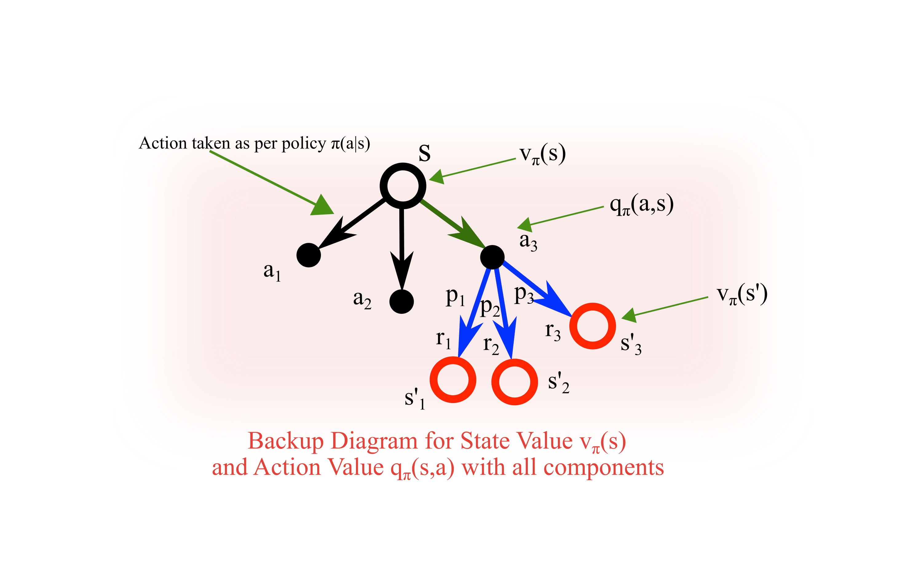
Another important concept is the backup diagram, which visualizes the Bellman equation using the notation of Sutton and Barto
We call this operation a backup. Unlike a simulated transition, which moves forward from to a sampled , a backup updates information at using estimates or returns associated with later states. Dynamic programming and temporal-difference value methods explicitly use Bellman-style backups. Monte Carlo methods instead use sampled complete returns, while policy-gradient methods need not explicitly approximate a Bellman equation.
- Root (open circle, representing state): State .
- First branch: Policy .
- First node (solid circle, representing state-action pair): Pair .
- Second branch: Environment dynamics .
- Leaves: Next state , whose value contributes to the backup at the current state .
5. Bellman Optimality Equation
We have defined value functions for a specific policy . But we don’t just want to evaluate a policy; we want to find the best policy (the Optimal Policy).
A policy is defined to be better than or equal to policy if its expected return is greater than or equal to that of for all states . In other words:
For a finite discounted MDP, there exists at least one stationary deterministic policy whose value is maximal in every state. Any such policy is an optimal policy, denoted by
All optimal policies share the same state-value function, called the optimal state-value function:
Similarly, optimal policies share the same optimal action-value function:
Just like the value function for a specific policy , the value function for the optimal policy can be written in a Bellman form, called the Bellman Optimality Equation.
The relationship between optimal action-value and optimal state-value is:
Bellman Optimality Equation for state-value function:
Bellman Optimality Equation for action-value function:
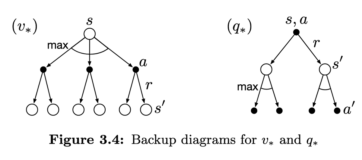
The arc between branches represents maximizing over actions instead of averaging them under a fixed policyWhy is the Bellman optimality equation harder to solve? For a fixed policy, the Bellman expectation equation is a linear system; see Appendix D. Maximizing over actions makes the optimality operator nonlinear, so the same direct linear solve does not apply. Standard alternatives include value iteration, policy iteration, and a linear-programming formulation. Q-learning estimates from samples when the dynamics are unavailable. See Appendix E..
Two boundary checks make the equations easier to interpret:
- If , then is only the expected immediate reward under .
- For an absorbing terminal state with zero subsequent reward, both its state value and every permitted terminal action value are zero.
6. References
- [Achiam, 2018]Spinning Up in Deep Reinforcement Learning[HTML]Achiam, Joshua, 2018.
- [Sutton et al., 2018]Reinforcement Learning: An Introduction[HTML]Sutton, Richard S. and Barto, Andrew G., 2018. The MIT Press.
- [Watkins et al., 1992]Q-learning[DOI]Watkins, Christopher J. C. H. and Dayan, Peter, 1992. Machine Learning, vol. 8, pp. 279--292
- [Alekh Agarwal et al., 2021]Reinforcement Learning: Theory and Algorithms[HTML]Alekh Agarwal, Nan Jiang Sham, M. Kakade and Wen Sun, 2021.
- [Vazquez-Reina]Deriving Bellman Equation in Reinforcement Learning[HTML]Amelio Vazquez-Reina (https://stats.stackexchange.com/users/2798/amelio-vazquez-reina). Cross Validated.
- [krishnab]How to setup the Bellman Equation as a linear system of equation[HTML]krishnab (https://cs.stackexchange.com/users/17922/krishnab). Computer Science Stack Exchange.
Appendix
A. Proof of Bellman Equation for State-Value Function
We have:
There are two expectations we need to resolve: the expectation of the immediate reward and the expectation of the next return .
Expectation of the next reward:
We have:
We need to “decompose” the probability into two parts: the policy and the dynamics . Applying the sum rule and product rule, we get:
Substituting this back into the expectation:
Once and are fixed, does not vary with or . We can therefore move it outside those sums and rearrange the finite sums:
Expectation of the return at the next time step:
Applying the law of total expectation, , we get:
Further expanding the conditional expectation:
Here we also use the fact that is a stationary Markov policy: after we condition on , future actions depend on rather than on the earlier state, action, or reward. Together with the Markov property of the dynamics, this lets us remove , , and from the inner conditional expectationConditional Independence: If , we say and are conditionally independent given .:
Combining everything, we arrive at:
B. Proof of Bellman Equation for Action-Value Function
From the proof in Appendix A, we see:
Also:
To satisfy the recursive nature of the Bellman equation, we need to express in terms of another . First:
The state name is only a dummy variable, so the same identity at the successor state is
Substituting this identity into gives the final result:
We can write the state-value function as a sum over action-value functions :
C. Unified Notation for Episodic and Continuing Tasks
In an episodic task, the interaction stops when we reach a terminal state. But our continuing-task equations are easier to reuse if every state has a next transition. We can bridge the two views by extending the process after termination in a harmless way.
Let contain the non-terminal states and let include an absorbing terminal state . We give this state one dummy action, , and define:
What does this convention buy us?
- Once the process reaches , it stays there.
- Every later reward is zero, so extending the trajectory does not change the episodic return.
- The terminal value is therefore .
The dynamics now remain normalized even at the terminal state:
This is a notational extension, not a claim that the real environment continues after the episode ends.
D. Linearity of the Bellman Equation
For each state , we have a value . If we assume states, we can write equations, turning the task of finding into solving a system of equations:
Writing this system in matrix form shows that the Bellman equation for a specific policy is linear. First, define:
- State-transition matrix : If the agent is in state , what is the probability of transitioning to state , averaged over the actions of policy ?
- Expected reward vector : If the agent is in state , what is the expected reward, averaged over the actions of policy ?
Thus, the Bellman equation becomes:
Writing this as a system:
Finally, the matrix form is:
If , then is a stochastic matrix with spectral radius at most . Therefore, is invertible, and we can solve:
Notice how the condition matters here. If we include our absorbing state and set , the full transition matrix has eigenvalue , so is singular. For an episodic problem, we instead impose and solve over the transient non-terminal states when the policy reaches termination with probability .
Even when the inverse exists, we normally solve the linear system rather than explicitly forming the inverse. A direct dense solve costs roughly , although sparse or iterative solvers may do much better. More fundamentally, large state spaces make the system expensive, and model-free settings do not give us or in the first place.
E. How to Find the Optimal Policy
Suppose we already know . At each state, let be any action attaining the maximum in the Bellman optimality equation:
We use because several actions may tie. Setting gives a deterministic greedy policy, and in the finite discounted setting that policy is optimal.
There are two equivalent ways to make this choice: one uses and the dynamics, while the other uses directly.
Based on optimal state-value function:
- To find knowing , we must know the environment dynamics . We must also perform a one-step (look-ahead) search, summing over all possible next states and rewards .
- This selection appears greedy because we only look at the immediate reward and the value of the next state . However, this yields the optimal result for the long term. This works because already accounts for the optimal reward sequence in the future.
Based on optimal action-value function: If is already known, the agent does not need a one-step search; it can pick an action with the highest . The decision itself does not require an explicit dynamics model, although learning or computing still requires information obtained from a model or experience.