PapersTransformers are RNNs: Fast Autoregressive Transformers with Linear Attention
Page/ 17
100%
0 open
You may wonder what is a receptive field in a transformer. It is the size of the region in the input that produces (or influences) the feature. In transformer, we can think it as the number of tokens that the attention mechanism can attend to. With unmasked (non-causal) attention, one layer already has access to all N positions; with causal attention, position i has access only to positions at or before i. Read more in this blog post.
But why is it quadratic? Let’s recall the formula of causal self-attention:
O=softmax(dQKT+M)V
in which M is a binary mask that indicates which positions are allowed to attend to, for forbidden positions, we set the corresponding entry to negative infinity. d is the dimension of the query and key vectors.
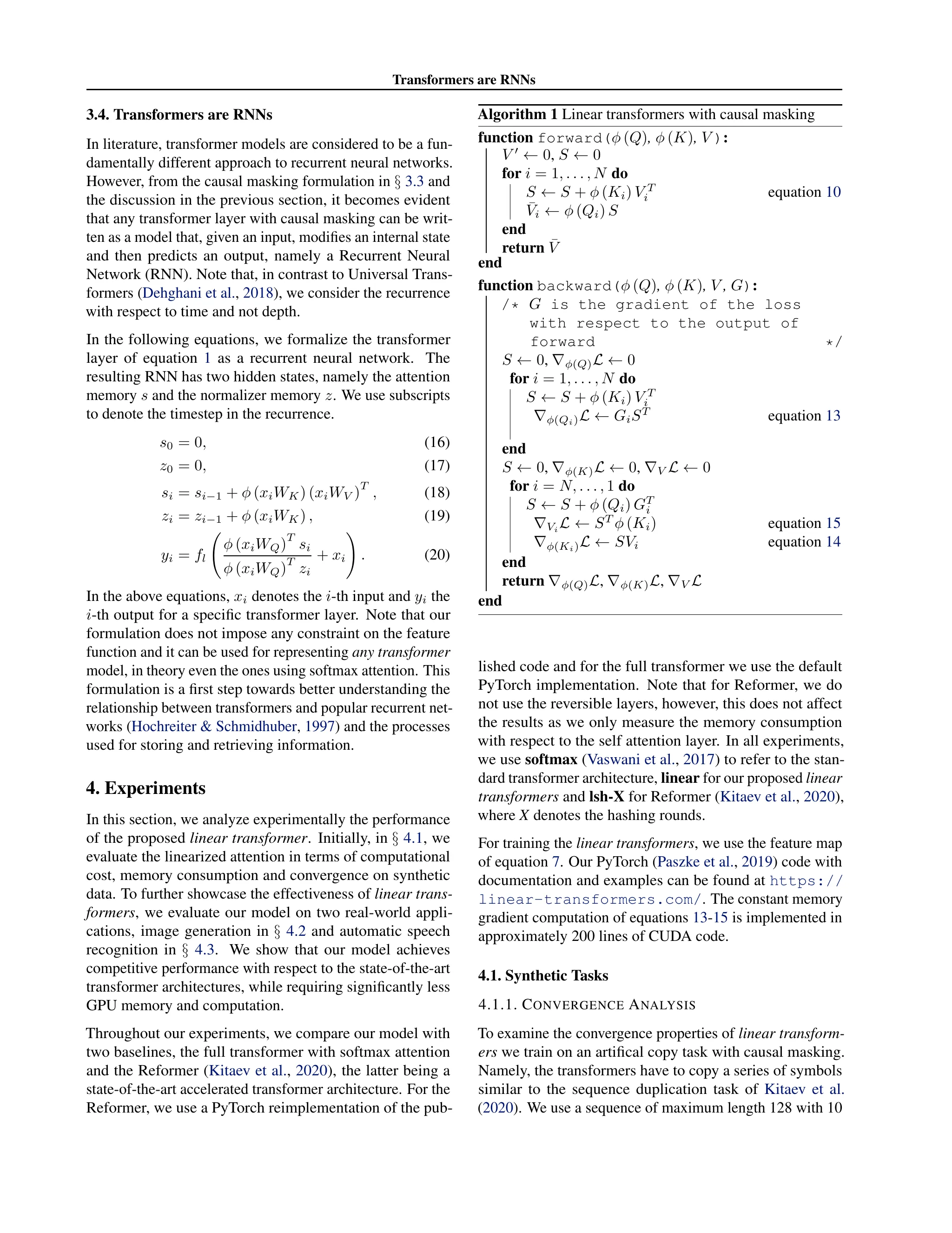
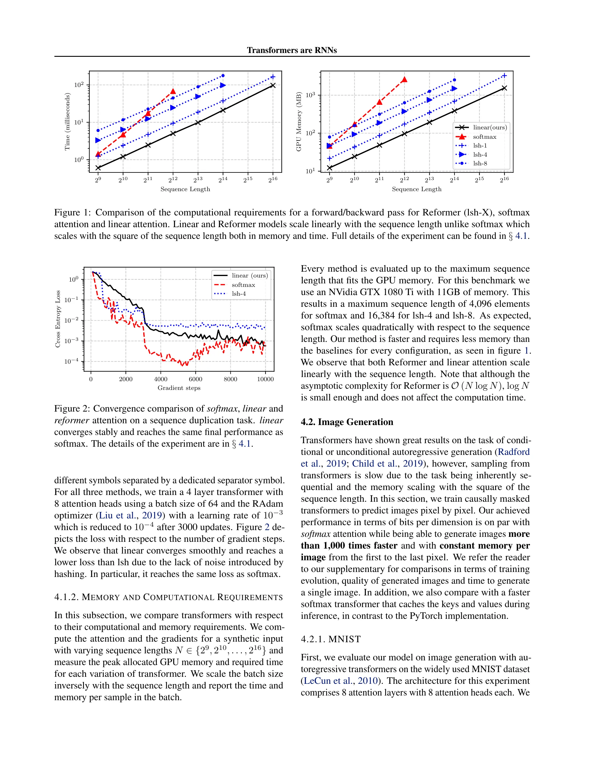
First, to calculate O we need to materialize QKT (this has been addressed in Flash Attention [Dao et al., 2022] where they compute the attention matrix in tiles without writing it to memory directly). The matrix Q and K both have shape N×d so QKT will have shape N×N and it occupies N2 in memory.
Same as this, calculating QKT is basically a matrix multiplication so the time complexity is O(N2d) but when we treat d as a constant, then when N grows, d becomes negligible and the final time complexity is O(N2).
In classic self-attention, the quadratic bottleneck causes the context to be limited. However, with the recent advances in long-context training, we can now have transformers with millions of context tokens and the context is still a limitation but we have raised the limit. Read more in this survey.
In LLM context, N is number of tokens and F is the hidden dimension. The formula is a little bit differnt, we can think each transformer layer as follow (using the pre-norm convention as in [Jurafsky et al., 2025]):
ylTl(⋅)=Al(LN(x))+x=MLP{LN(yl)}+yl
where LN is layer norm.
Even though the author used a different convention but the main contribution is in the self-attention equation not the whole transformer.
From the matrix form, we have a vector form of V′, let’s call it Vi′, we have:
Note that the denominator of softmax is independent of j so we can move it outside the sum to get the second equation. Also, when factoring out the denominator, I have changed the index from n to j to match the numerator.
If we let sim(Qi,Kj)=exp(QiTKj/D) then we have:
Vi′=∑j=1Nsim(Qi,Kj)∑j=1Nsim(Qi,Kj)Vj
You might wonder why they choose an inner-product kernel?
Actually, we want to choose a feature map ϕ such that sim(Qi,Kj)=ϕ(Qi)Tϕ(Kj). Because sim can be represented as an inner-product kernel therefore we can use reassociating trick to compute the attention matrix in linear time (will see the reason soon).
Why can we reassociate the attention computation without changing its output? Let each query and key be column vectors with shape C×1, where C is the feature-map dimension. For the value, it is a column vector with shape M×1, where M is the value dimension.
You can see that this is the result of matrix multiply with a column vector where ai1,...,aiC are the elements of column vector ai and ∑j=1Nbj1cj,...,∑j=1NbjCcj are the column of some matrix, only need to find that matrix. Continue on the derivation:
This will have some confusion but the second Vi′ is actually a row vector not a column vector as in Eq(4).
Now we move to the derivation of Eq(6). Let:
A=ϕ(Q)∈RN×C,B=ϕ(K)∈RN×C,V∈RN×M,
where ai, bj, and vj are rows of A, B, and V. For query i, the numerator is the row vector:
ui=j=1∑N(aibjT)vj∈R1×M.Warning
As in previous note, we will use the convention of row vectors. Because using row vector, we need to change ϕ(Qi)Tϕ(Kj) to ϕ(Qi)ϕ(Kj)T to get the correct result (or otherwise, it would be an outer product instead of inner product).
To obtain all ui at once, consider entry (i,m) of (ABT)V: