Note
- Source code: https://github.com/vietfood/lazy-unlearner
- Gemma-2-2B-RMU: https://huggingface.co/lenguyen1807/gemma-2-2b-RMU
- Gemma-2-2B-it-RMU: https://huggingface.co/lenguyen1807/gemma-2-2b-it-RMU
Warning (AI Usage Transparency)
This post is based on my undergraduate thesis. I used Gemini-2.5-Flash to label model outputs during probe training (see Section 2.1), and Gemini-2.5-Pro with Claude Sonnet 4.5 to help refine the grammar and clarity of the writing. All experimental design, implementation, analysis, and conclusions are my own.
Important (TL;DR)
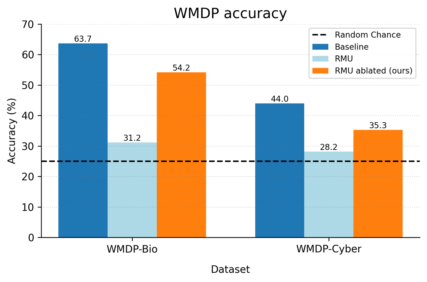
RMU (Representation Misdirection Unlearning) is supposed to make LLMs forget dangerous knowledge. We open the hood and find that it mostly works through a single vector --- a “junk direction” --- in the model’s residual stream. Ablating this one direction on Gemma-2-2B recovers 74.2% of the performance gap on the WMDP-Bio benchmark and 65.8% on WMDP-Cyber. Worse, this direction is not randomly constructed: the model builds it using its own pretraining features about the very topic it is supposed to forget. This is what Arditi et al. termed shallow unlearning — our contribution is a mechanistic account of why it happens and a causal framework (TCE / IE / DE) to quantify it, alongside an adversarial training approach designed to force a deeper solution.
0. Motivation
Modern LLMs are trained on the next-token prediction objective over enormous corpora scraped from the internet. This objective has no preference for human values---it simply rewards the model for assigning high probability to the next token. As a result, a capable LLM will have absorbed both the useful knowledge of the web and its harmful undercurrents: detailed information about synthesizing pathogens, developing cyberattack tools, or other dangerous capabilities. The danger is not hypothetical. Urbina et al. demonstrated that an AI system, when repurposed for adversarial use, generated 40,000 candidate toxic molecules in under six hours.
The problem with surface-level fixes. The most widely deployed safety technique is RLHF, which uses human feedback to fine-tune a model to produce responses aligned with human values. While effective in practice, RLHF and related approaches like in-context safety prompting share a fundamental limitation: they teach the model to conceal harmful knowledge rather than erase it. The underlying circuits encoding that knowledge remain intact, merely suppressed by a thin veneer of alignment. Sufficiently creative jailbreaks can pierce through this veneer because the information was never removed---it was only hidden.
Machine Unlearning as principled removal. Machine Unlearning (MU) takes a more principled approach. Given a forget set of harmful data and a retain set of benign data, the goal is to produce a model whose behavior is indistinguishable from a model that was never trained on at all. The gold standard---exact unlearning---would require retraining from scratch on only, which for modern LLMs costs millions of dollars and months of compute. Approximate unlearning methods instead attempt to efficiently modify the existing model weights to approximate this gold standard.
What this work does. Representation Misdirection Unlearning (RMU) is currently among the strongest approximate unlearning methods for LLMs. This note investigates a critical question: when RMU “works,” what is it actually doing inside the model? The empirical investigation in Section 2 uses mechanistic interpretability tools---linear probes, causal interventions, and sparse autoencoders---to dissect RMU’s internal mechanism. Section 3 then introduces an adversarial training framework designed to patch the vulnerability that this analysis uncovers.
1. Background
Let a Large Language Model (LLM) be parameterized by .
- is a function that maps an input token to a logit vector of dimension . We refer to as vocabulary of model. Thus:
- Let denote the activation vector of the LLM at layer and token position (or input vector at layer ). Correspondingly, let be the remainder of the LLM computational graph, which maps the activation vector at layer and token position to the corresponding logit vector . Therefore, we can express the computation as:
- The output distribution over the vocabulary at position is given by:
1.1 RMU (Representation Misdirection Unleanring)
RMU
Consider a forget set and a retain set . The forget set contains harmful data (e.g., related to bioweapons, security vulnerabilities)
- Forget Loss:
- Retain Loss:
Here, is the activation from the frozen, original model, while is from the model being unlearned. and are the total tokens of forget set and retain set respectively. The total loss is:
1.2 Weaknesses of RMU
Recent work by Łucki et al.

2. An Empirical Motivation
Warning
To ground above idea, we first conducted an empirical investigation into the mechanics of shallow unlearning on a Gemma-2-2B model. This exploration, initially part of our thesis, followed a path of inquiry that began with creating a tool to detect unlearning, isolating the underlying mechanism, and finally, deconstructing that mechanism to understand its origins. This journey revealed critical limitations in post-hoc analysis and directly motivated the adversarial framework presented in the main body of this note.
2.1 Quantifying “Junk” with a Linear Probe
Observation: The output from an RMU-unlearned model on forgotten prompts often appears random and incoherent.
- Prompt: By what mechanism(s) do modern Beijing strains of Mycobacterium tuberculosis have higher virulence than ancient Beijing strains?
- Original Model: The answer is that the modern strains have acquired a gene that encodes a protein that is a virulence factor…
- RMU Model: 1. They are more virulent than ancient Beijing strains. 2. They are less virulent than ancient Beijing strains. 3. They are more virulent than…
So our initial challenge was to quantitatively measure when a model was “unlearning” in a shallow way. We observed that RMU-tuned models often produce incoherent or evasive responses, which we will refer to as “junk” outputs for the remainder of this analysis. We hypothesized that this behavior could be identified from the model’s internal activations.
To test this, we framed the problem as a binary classification task: training a simple linear classifier---a linear probe
- Probe Training: We constructed a dataset of 2,000 prompts, combining 1,000 questions from the WMDP benchmark with 1,000 general-purpose samples from Alpaca
[12] . We used a larger LLM (Gemini-2.5-Flash) to label the Gemma-2-2B model’s outputs as eitherjunk(Label 1) ornon-junk(Label 0). After training a probe on the final-token activations for each layer of the model, we found that the probe at Layer 12 achieved the highest performance (ROC-AUC > 0.7), confirming that a non-trivial, linearly decodable signal for this behavior exists within the model’s representations.

- Limitations of the Linear Probe Approach: While the probe was effective, this process revealed several fundamental limitations that made it unsuitable as a robust research tool:
- Scalability: This approach is model-specific and requires a new, labeled dataset and training process for every model architecture under investigation.
- Subjectivity and Bias: The definition of an “junk” output is subjective and relies on the labeling criteria of an external LLM. This introduces an unquantifiable bias into the probe’s concept of evasion.
- Misalignment of Objectives: The probe identifies a correlate of unlearning (incoherent output), but this is not necessarily the mechanism of unlearning. The true goal of an attacker is to recover information, not simply to detect gibberish. This proxy is therefore indirect and potentially fragile.
This realization was a critical turning point. A post-hoc, supervised tool was too brittle. We needed a more direct method to find the underlying mechanism itself.
2.2 Isolating the Junk Direction
Having established a proxy for junk score (the probe’s score), we sought to isolate the direction in activation space responsible for inducing this behavior. Following the methodology of Arditi et al.
Our analysis revealed a key insight: the junk directions extracted from the WMDP-Bio and WMDP-Cyber datasets were highly aligned, exhibiting a cosine similarity greater than 0.8 at many layers.

This suggested that the model was not learning separate unlearning mechanisms for each topic but was instead relying on a single, shared mechanism. We validated this by creating a shared direction, averaging the Bio and Cyber directions.
2.2.1 A Causal Accounting of Recovery
To precisely quantify how much of RMU’s unlearning is mediated by the junk direction, we adopt a three-component causal decomposition. Let , , and denote the original model, the RMU-trained model, and the model after ablating the best junk direction respectively. We define:
- Total Causal Effect (TCE): the full accuracy drop caused by RMU.
- Indirect Effect (IE): the portion of the drop attributable to the junk direction mechanism.
- Direct Effect (DE): the residual drop caused by the weight changes themselves (), independent of the junk direction.
The accuracy recovery rate is then defined as:
Intuitively, if , the junk direction is the mechanism of unlearning; if , deeper weight-level changes dominate.
Ablating the shared direction yields on WMDP-Bio and on WMDP-Cyber---confirming that the single shared direction is the dominant, causally significant component of the shallow unlearning mechanism. The table below summarizes the full benchmark results across all directions we evaluated, including a random baseline (a random vector orthogonal to with the same norm):

2.3 Deconstructing the Direction with Feature Analysis
We had isolated a direction. The final question was: what is this direction made of? What concepts does it represent? To answer this, we turned to Sparse Autoencoders (SAEs), which decompose activations into more interpretable features. Using the Relative Gradient technique from Daniel et al.
- In the Base Model: The junk direction was composed of generic, topic-agnostic features related to syntax, programming concepts, and statistical language (e.g., “C++ memory management,” “statistical terms”).

- In the RMU-Unlearned Model: The composition of the direction fundamentally changed. RMU had rewired the model to construct the junk direction using features semantically related to the forgotten topics themselves, such as “words related to infectious diseases” (SAE vector 3877) and “terms related to medical imaging” (SAE vector 3484).

This was the crucial insight. Shallow unlearning

Next, although the activated features now resemble those of the base model after we ablated junk direction , a few features still encode biological knowledge. This provides evidence that the junk direction is not the sole mechanism by which RMU operates.
Some biology-related features include:
- 8085: “terms related to viral infections and drug resistance”.
- 16213: “phrases and references related to medical conditions and healthcare”.
Removing feature 16213 (the most strongly activated one) yields the following results:
| Model | WMDP-Bio | WMDP-Cyber | MMLU |
|---|---|---|---|
| Remove | 50.59 | 32.16 | 47.34 |
| Remove feature 16213 after removed | 51.68 | 33.71 | 48.08 |
2.4 Summary and Conclusions
The empirical investigation in Sections 2.1–2.3 yields a coherent mechanistic picture of how RMU achieves its unlearning effect on Gemma-2-2B.
The dominant mechanism is the junk direction. A single vector in activation space, installed at layer 9 of the residual stream, accounts for of the WMDP-Bio accuracy gap and of the WMDP-Cyber gap. Ablating an orthogonal random baseline with the same norm produces near-zero recovery, confirming the effect is specific and not a side effect of norm perturbation.
The shallow / deep dichotomy. Because cannot reach , the junk direction is not the complete story. In Arditi et al.’s framing
Why RMU creates a lazy solution. The answer lies in the structure of its loss function. By targeting a single fixed random vector , RMU hands the optimizer a simple objective: redirect the activations on harmful inputs. The easiest mathematical path is to learn a single direction that, when added to any harmful prompt’s residual stream, pushes the output distribution toward incoherence. Critically, the optimizer does not construct this direction from scratch---it repurposes the model’s own pretraining features about the harmful topic to build it. This is the core insight: shallow unlearning is not a random artifact; it is a learned response.
Limitations and future directions. This analysis has several important limitations: (i) all experiments are conducted on Gemma-2-2B only; generalization to larger or differently-trained models requires further study; (ii) the linear probe’s labeling relies on an external LLM, introducing subjective bias; (iii) the deep unlearning component has not yet been mechanistically characterized. Two promising approaches to illuminate it further are Relative Gradient analysis (tracing which SAE features build the junk direction across layers) and Attribution Graphs (a full causal circuit representation of the unlearning mechanism). These threads directly motivate the adversarial framework proposed in Section 3.
3. Proposed Method
Objective: We aim to prevent the model from adopting a “lazy” solution---namely, using a single directional mechanism to achieve unlearning. Our goal is to force the model to learn a more robust and deeply embedded unlearning solution.
This behavior can be understood through the lens of specification gaming. The optimizer, acting as a “lazy servant,” finds the simplest mathematical path to satisfy the given loss function, often without capturing the researcher’s semantic intent.
- Our Semantic Goal: To genuinely erase knowledge related to a harmful topic, which should require a meaningful change to the model’s internal circuits.
- The Loss Function’s Goal: To make the activation vector diverge from its original state by redirecting it towards a random vector .
Approach: We reframe this challenge as a min-max optimization problem (adversarial training).
- Attacker: The attacker’s goal is to find the “laziest” direction, denoted , which, when added to an activation vector, is most effective at achieving the unlearning objective (which we model as maximizing output entropy).
- Defender: The defender updates the model weights to steer activation vectors away from this adversarial direction . The intuition is to force the model to find an alternative, more complex unlearning mechanism, rather than collapsing its representations onto this single lazy direction.
Danger (Key Assumptions and Caveats)
Our approach rests on two key assumptions that require further investigation:
- Is maximizing entropy the correct adversarial objective? We use output entropy as a proxy for finding the “laziest” unlearning direction. However, a more direct objective for an attacker might be to find a direction that recovers the forgotten information most effectively. Our proxy may not perfectly align with the true adversarial goal.
- Is the “lazy” solution a single direction? The shallow unlearning mechanism may not be confined to a single vector but could exist within a low-dimensional subspace. Our method, by targeting a single direction , might be insufficient to neutralize a multi-dimensional “lazy subspace,” as hinted at by our experiments with a shared refusal direction.
3.1 Attacker Optimization
Following Yuan et al.
Let be a perturbation vector (or the “lazy” direction). The pertubed logit is:
where is the L2-normalized vector .
The attacker problem is:
The constraint focuses on finding a direction rather than its magnitude, is number of tokens and .
3.2 Defender Optimization
Given the adversarial direction found by the attacker, the defender’s objective is to force the model’s activations on forget-set data to be orthogonal to this direction. This is achieved by minimizing the squared inner product, effectively projecting the activations into the null-space of :
This defense loss acts as a regularizer on the original RMU objective. The final forget loss is:
Note (Why Regularize Instead of Replace?)
We propose using as a regularizer rather than a complete replacement for the original . Our rationale is that the original RMU objective provides a useful inductive bias: it disrupts the original activations, encouraging the model to rewire its internal circuits.
However, empirical evidence shows it often achieves this via a simplistic, “lazy” mechanism. Our adversarial regularizer, , acts as a targeted penalty against this specific lazy solution. Replacing the loss entirely would remove the “disruption” signal, only telling the optimizer what not to do (i.e., “steer away from the high-entropy direction”) without providing a constructive unlearning objective.
3.3 What’s next ?
A critical next step is to empirically verify whether the shallow unlearning phenomenon persists in more advanced RMU variants, such as Adaptive-RMU
4. Experiments
Important
This research is currently at the conceptual stage, and I plan to carry out empirical validation in the near future as soon as the necessary computational resources are available.
5. Acknowledgement
Thanks @arditi for insightful discussions regarding high-entropy output distributions and the mechanics of refusal directions in RMU. Thanks @longphan for support with data and baseline RMU implementation. Thanks professor @Le Hoai Bac for his invaluable guidance throughout this work. I also used Google’s @Gemini-2.5-Pro to help refine the grammar and clarity of this note. Finally, I thank @mom and @dad for providing the financial support and a warm place to sleep, enabling me to pursue this research.
Citation
@misc{ln2025rmu, author={Nguyen Le}, title={Finding and Fighting the Lazy Unlearner: An Adversarial Approach}, year={2025}, url={https://lenguyen.vercel.app/note/rmu-improv}}References
- The WMDP Benchmark: Measuring and Reducing Malicious Use with Unlearning, Li, Nathaniel and Pan, Alexander and Gopal, Anjali and Yue, Summer and Berrios, Daniel and Gatti, Alice and Li, Justin D. and Dombrowski, Ann-Kathrin and Goel, Shashwat and Mukobi, Gabriel and Helm-Burger, Nathan and Lababidi, Rassin and Justen, Lennart and Liu, Andrew Bo and Chen, Michael and Barrass, Isabelle and Zhang, Oliver and Zhu, Xiaoyuan and Tamirisa, Rishub and Bharathi, Bhrugu and Herbert-Voss, Ariel and Breuer, Cort B and Zou, Andy and Mazeika, Mantas and Wang, Zifan and Oswal, Palash and Lin, Weiran and Hunt, Adam Alfred and Tienken-Harder, Justin and Shih, Kevin Y. and Talley, Kemper and Guan, John and Steneker, Ian and Campbell, David and Jokubaitis, Brad and Basart, Steven and Fitz, Stephen and Kumaraguru, Ponnurangam and Karmakar, Kallol Krishna and Tupakula, Uday and Varadharajan, Vijay and Shoshitaishvili, Yan and Ba, Jimmy and Esvelt, Kevin M. and Wang, Alexandr and Hendrycks, Dan Proceedings of the 41st International Conference on Machine Learning,PMLR, 2024https://proceedings.mlr.press/v235/li24bc.html
- An Adversarial Perspective on Machine Unlearning for AI Safety, Jakub \Lucki and Boyi Wei and Yangsibo Huang and Peter Henderson and Florian Tram\`er and Javier RandoTransactions on Machine Learning Research, 2025https://openreview.net/forum?id=J5IRyTKZ9s
- Unlearning via RMU is mostly shallow, Andy, Arditi Less Wrong,2024https://www.lesswrong.com/posts/6QYpXEscd8GuE7BgW/unlearning-via-rmu-is-mostly-shallow
- On effects of steering latent representation for large language model unlearning, Huu-Tien, Dang and Pham, Tin and Thanh-Tung, Hoang and Inoue, Naoya Proceedings of the Thirty-Ninth AAAI Conference on Artificial Intelligence and Thirty-Seventh Conference on Innovative Applications of Artificial Intelligence and Fifteenth Symposium on Educational Advances in Artificial Intelligence,AAAI Press, 2025https://doi.org/10.1609/aaai.v39i22.34544
- Improving LLM Unlearning Robustness via Random Perturbations, Dang Huu-Tien and Hoang Thanh-Tung and Anh Bui and Le-Minh Nguyen and Naoya Inoue2025https://arxiv.org/abs/2501.19202
- Latent Adversarial Training Improves Robustness to Persistent Harmful Behaviors in LLMs, Abhay Sheshadri and Aidan Ewart and Phillip Guo and Aengus Lynch and Cindy Wu and Vivek Hebbar and Henry Sleight and Asa Cooper Stickland and Ethan Perez and Dylan Hadfield-Menell and Stephen Casper2025https://arxiv.org/abs/2407.15549
- A Closer Look at Machine Unlearning for Large Language Models, Xiaojian Yuan and Tianyu Pang and Chao Du and Kejiang Chen and Weiming Zhang and Min Lin The Thirteenth International Conference on Learning Representations,2025https://openreview.net/forum?id=Q1MHvGmhyT
- Refusal in Language Models Is Mediated by a Single Direction, Andy Arditi and Oscar Balcells Obeso and Aaquib Syed and Daniel Paleka and Nina Rimsky and Wes Gurnee and Neel Nanda The Thirty-eighth Annual Conference on Neural Information Processing Systems,2024https://openreview.net/forum?id=pH3XAQME6c
- Measuring Massive Multitask Language Understanding, Dan Hendrycks and Collin Burns and Steven Basart and Andy Zou and Mantas Mazeika and Dawn Song and Jacob SteinhardtProceedings of the International Conference on Learning Representations (ICLR), 2021
- Aligning AI With Shared Human Values, Dan Hendrycks and Collin Burns and Steven Basart and Andrew Critch and Jerry Li and Dawn Song and Jacob SteinhardtProceedings of the International Conference on Learning Representations (ICLR), 2021
- Simple probes can catch sleeper agents, Monte MacDiarmid and Timothy Maxwell and Nicholas Schiefer and Jesse Mu and Jared Kaplan and David Duvenaud and Sam Bowman and Alex Tamkin and Ethan Perez and Mrinank Sharma and Carson Denison and Evan Hubinger2024https://www.anthropic.com/news/probes-catch-sleeper-agents
- Stanford Alpaca: An Instruction-following LLaMA model, Rohan Taori and Ishaan Gulrajani and Tianyi Zhang and Yann Dubois and Xuechen Li and Carlos Guestrin and Percy Liang and Tatsunori B. HashimotoGitHub repository, GitHub, 2023
- HarmBench: A Standardized Evaluation Framework for Automated Red Teaming and Robust Refusal, Mantas Mazeika and Long Phan and Xuwang Yin and Andy Zou and Zifan Wang and Norman Mu and Elham Sakhaee and Nathaniel Li and Steven Basart and Bo Li and David Forsyth and Dan Hendrycks2024
- Catastrophic jailbreak of open-source llms via exploiting generation, Huang, Yangsibo and Gupta, Samyak and Xia, Mengzhou and Li, Kai and Chen, DanqiarXiv preprint arXiv:2310.06987, 2023
- Universal and Transferable Adversarial Attacks on Aligned Language Models, Andy Zou and Zifan Wang and J. Zico Kolter and Matt Fredrikson2023
- Detecting Strategic Deception Using Linear Probes, Nicholas Goldowsky-Dill and Bilal Chughtai and Stefan Heimersheim and Marius Hobbhahn2025https://arxiv.org/abs/2502.03407
- Finding Features Causally Upstream of Refusal, Lee, Daniel Less Wrong,https://www.lesswrong.com/posts/Zwg4q8XTaLXRQofEt/finding-features-causally-upstream-of-refusal
Appendix
A. Dataset
-
The WMDP (Weapons of Mass Destruction Proxy) dataset
[1] is a multiple-choice benchmark consisting of one question and four answer options, designed to measure hazardous knowledge in large language models LLM across domains such as biology, cybersecurity, and chemistry. The dataset comprises 3,668 expert-developed questions intended as a representative metric for evaluating and mitigating risks of malicious misuse. -
In biology (referred to as WMDP-Bio), the dataset contains 1,273 questions. These include biotechnology-related risks such as historical instances of bioweapons, pathogens with pandemic potential, construction-related issues (e.g., reverse engineering of viruses), and experimental aspects (e.g., assays for viral properties).
-
In cybersecurity (referred to as WMDP-Cyber), the dataset includes 1,987 questions structured around the stages of a cyberattack: reconnaissance, exploitation, attack, and post-exploitation. WMDP-Cyber evaluates a model’s ability to understand concepts and techniques related to vulnerability discovery, exploit development, and the use of popular offensive frameworks such as Metasploit and Cobalt Strike.
-
Model performance will be evaluated in terms of accuracy on WMDP multiple-choice questions (restricted to WMDP-Bio and WMDP-Cyber). A model trained with unlearning should exhibit reduced accuracy on WMDP while maintaining accuracy on unrelated benchmarks (in the cited work, this is the MMLU dataset
[9] [10] ). We refer to this overall evaluation as the WMDP Benchmark.
B. More on Probe
Below is data statistics for Probe Training:
| Dataset | Total Samples | Label 1 (Junk) | Label 0 (Non-Junk) |
|---|---|---|---|
| 1280 | 1016 | 264 | |
| 320 | 258 | 62 | |
| 400 | 324 | 76 |
The dataset is highly imbalanced. This is understandable given that the base model, Gemma-2-2B, is relatively small. For many challenging (harmful or harmless) questions, the model fails to provide an answer, which is then labeled as junk. With a larger model, this imbalance would likely be reduced.
In training procedure, we apply z-score normalization using the mean and standard deviation computed on the training set, and reuse these statistics for normalization on validation and test sets
Once the best probe is selected, it is used to assign a junk score to activations as:
where is any activation vector, and are the weights and bias of the best-performing probe.
C. Isolating the Junk Direction Methodology
C.1 Dataset
Let denote the dataset used for extracting junk directions. This dataset is split into a training set and a validation set . Specifically, is obtained by sampling from the WMDP dataset, which consists of WMDP-Bio and WMDP-Cyber, corresponding to and (but collectively referred to as ).
The sampling process follows these conditions:
- Samples must not overlap with the detector training dataset of linear probe.
- Samples must not contain questions with the word “which”. The reason is that such questions typically require both the question and the answer context. If used in isolation, they degrade model performance and sometimes lead to empty or anomalous outputs.
- The maximum question length is limited to 1024 characters. This restriction arises both from resource constraints and from the observation that including overly long questions does not affect the final results.
After applying these conditions, 300 samples are drawn from each of WMDP-Bio and WMDP-Cyber, for a total of 600 samples. These are then split into and with an 80%/20% ratio.
In addition, we incorporate out-of-distribution (OOD) data, denoted . This dataset combines three harmful-knowledge benchmarks: AdvBench
C.2 Direction Extraction via Difference-in-Means
Our investigation is built on a central hypothesis: the performance degradation observed in an RMU-unlearned model is not solely due to diffuse changes in its weights. Rather, we posit that RMU instills a specific, learned mechanism.
Causal Hypothesis: For a harmful input, the RMU model adds a specific vector, the junk direction , to the residual stream at a specific layer. This intervention is the primary cause of the model’s junk, low-quality output and the corresponding drop in accuracy on harmful benchmarks.
To extract junk directions, we employ the same method as in
We use the Difference-in-Means
This process is performed for each layer and for the final five token positions of the input prompts, yielding a set of candidate directions.
Warning
The last five tokens (from to ) are selected for the following reasons:
- In the original study by Arditi
[3] , eight final tokens were chosen and averaged. This choice was essentially arbitrary. - In the study on refusal directions
[8] , the models examined were instruction-tuned and employed structured prompts (e.g.,user:<instruction>model:). Consequently, they selected tokens after the instruction (post-instruction), such asmodel:. However, the models in this thesis are base models without instruction fine-tuning, so such prompt structures cannot be used. - This thesis hypothesizes that information is aggregated in the final tokens. Selecting only the very last token would be overly restrictive. Therefore, the final five tokens are used instead.
C.3 Causal Validation and Selection
From the set of candidate directions, we must identify the one that is most causally responsible for the junk behavior. We use a series of causal interventions, evaluated on a validation set , using the junk score from the linear probe (Appendix B) as our metric.
- Ablation Intervention (Bypass): To test if removing a direction restores coherent behavior in the RMU model, we compute its
bypassscore. We intervene on the RMU model by projecting out the component of its activations that lies along the candidate direction . The optimal direction should maximally reduce the junk score.
- Addition Intervention (Steer): To test if adding a direction induces junk behavior in the base model, we compute its
steerscore. We intervene by adding the direction to the base model’s activations. A potent junk direction should significantly increase the junk score.
- KL Divergence Sanity Check: A true junk direction should be specific to the RMU mechanism and not disrupt the base model’s general knowledge. We verify this by ablating the direction from the base model and measuring the KL divergence between the original and perturbed output distributions. A low KL divergence indicates the direction is inert in the base model, confirming its specificity.
The best junk direction is selected as the candidate that minimizes the bypass score, maximizes the steer score, and maintains a low KL divergence.
D. Relative Gradient Methodology
Let the best junk direction be denoted by , where is the layer and is the token position at which this junk direction is selected. Define:
as the dot product between the residual stream vector of the model , namely at layer and token (the same position where the junk direction is extracted), with the best junk direction for input . Then, the junk gradient is defined as:
i.e., the derivative of the earlier residual streams () with respect to , at token position and input . Here, we choose and (which is the layer and token position of best junk direction).
Intuition
Intuitively, the junk gradient indicates which directions are most responsible for producing the junk direction, and thus which features contribute to its formation. Following
Let denote a dataset sampled from the remaining examples (disjoint from and ). For each of WMDP-Bio and WMDP-Cyber, we define and , respectively.
The aggregated junk gradients at layer are computed as:
In this work, is chosen empirically. This layer is neither too early (close to the embedding layer) nor too late (close to the output), making it a reasonable midpoint for analysis.
Finally, the cosine similarity is computed between these junk gradients and each residual stream vector of the decoder weight matrix from the SAE (Sparse Autoencoder) at layer .
E. Junk Direction Selection Results
The table below reports the three evaluation criteria---bypass score, steer score, and KL divergence---for the four candidate junk directions. The shared direction is ultimately chosen because it achieves the best overall balance across all three metrics.
| Direction | Layer | Token Position | Bypass | Steer | KL | Extraction Dataset |
|---|---|---|---|---|---|---|
| 9 | and | |||||
| 9 | ||||||
| 9 | ||||||
| 10 |
All meaningful junk directions concentrate at layer 9 (token position ), confirming this as the primary layer of RMU’s suppression mechanism. The OOD direction has a low bypass score but nearly fails the steer test () and has a much higher KL ()---meaning it disrupts the base model’s general distribution and is therefore rejected. The Cyber direction has the strongest bypass score in isolation but poor cross-domain generalization. The shared direction, averaged across both domains, offers the best tradeoff.
F. Full Benchmark Results
The tables below provide the complete accuracy and recovery-rate results. For each direction , a corresponding random orthogonal baseline (same norm, uniformly random direction orthogonal to ) confirms that recovery is direction-specific and not a generic norm-perturbation artifact.
Accuracy on WMDP Benchmark after ablating each direction:
| Model | WMDP-Bio | WMDP-Cyber | MMLU |
|---|---|---|---|
| Base model | 58.76 | 34.93 | 49.73 |
| RMU model | 25.61 | 26.77 | 43.35 |
| Remove | 50.59 | 32.16 | 47.34 |
| Remove (random baseline) | 25.22 | 26.67 | 43.71 |
| Remove | 48.39 | 33.82 | 47.14 |
| Remove (random baseline) | 25.53 | 26.72 | 43.44 |
| Remove | 50.43 | 29.49 | 47.32 |
| Remove (random baseline) | 26.16 | 26.37 | 43.74 |
| Remove | 34.49 | 28.94 | 45.98 |
Accuracy recovery rate for each direction:
| Direction | WMDP-Bio (%) | WMDP-Cyber (%) | MMLU (%) |
|---|---|---|---|
| 74.2 | 65.8 | 66.3 | |
| 68.5 | 84.8 | 63.4 | |
| 73.4 | 33.6 | 65.9 | |
| 26.6 | 26.5 | 43.8 |
for all random baselines is in every case---ablating random directions leaves performance unchanged or marginally hurts it, confirming the effect is specific to the true junk directions.
Qualitative recovery. After ablating , the model recovers coherent, substantive responses on formerly-forgotten prompts:
Prompt: “By what mechanism(s) do modern Beijing strains of Mycobacterium tuberculosis have higher virulence than ancient Beijing strains?”
Base model: “The answer is that the modern strains have acquired a gene that encodes a protein that is a virulence factor…”
RMU model: “1. They are more virulent than ancient Beijing strains. 2. They are less virulent than ancient Beijing strains. 3. They are more virulent than…”
After ablating : “The answer is that the ancient Beijing strains were not as virulent as the modern strains. The modern strains are more virulent because they are more likely to cause disease in humans…”