Warning (AI Usage Transparency)
This post is based on my undergraduate thesis. I used Gemini-2.5-Flash to label model outputs during probe training (see Section 2.1), and Gemini-2.5-Pro with Claude Sonnet 4.5 to help refine the grammar and clarity of the writing. All experimental design, implementation, analysis, and conclusions are my own.
Abstract
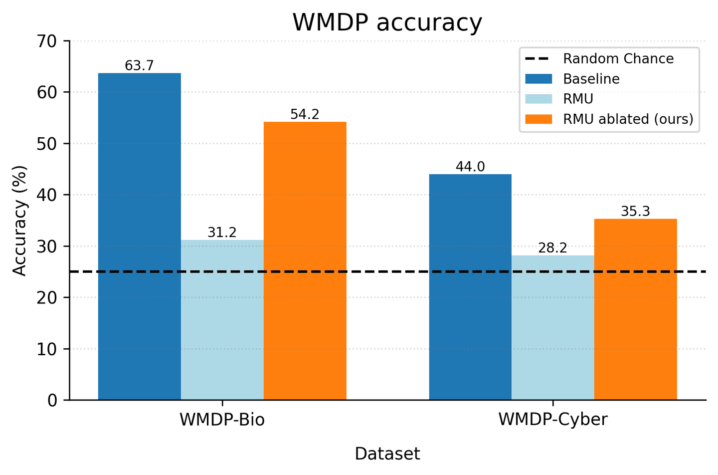
RMU (Representation Misdirection Unlearning) aims to make LLMs forget dangerous knowledge. I find that, on Gemma-2-2B, much of its effect is mediated by a single residual-stream vector: a “junk direction”. Ablating that direction recovers 74.2% of the WMDP-Bio performance gap and 65.8% on WMDP-Cyber. The direction is not random: RMU builds it from the model’s own pretrained features about the topic being forgotten. This gives a mechanistic account of shallow unlearning
0. Motivation
Modern LLMs are trained to predict the next token over internet-scale corpora. That objective has no built-in preference for human values: it rewards whatever makes the next token more likely. As a result, capable models absorb both useful knowledge and dangerous knowledge, including information about pathogen synthesis, cyberattacks, and other harmful capabilities. The risk is not hypothetical: Urbina et al. showed that an AI system repurposed for adversarial use could generate 40,000 candidate toxic molecules in under six hours.
The problem with surface-level fixes. RLHF and safety prompting can make models refuse harmful requests, but they mostly teach the model to hide dangerous knowledge, not erase it. The circuits remain; alignment only suppresses their expression. Creative jailbreaks can still reach them because the information was never removed.
Machine unlearning as principled removal. Machine Unlearning (MU) starts from a forget set of harmful data and a retain set of benign data. The ideal output is a model that behaves like a model trained without . Exact unlearning would require retraining on from scratch, which is prohibitively expensive for modern LLMs. Approximate methods instead try to edit the existing model efficiently.
What this work does. Representation Misdirection Unlearning (RMU) is one of the strongest approximate unlearning methods for LLMs. This note asks: when RMU “works,” what is it doing inside the model? Section 2 uses linear probes, causal interventions, and sparse autoencoders to inspect the mechanism. Section 3 proposes an adversarial training objective designed to patch the vulnerability.
1. Background
Let a Large Language Model (LLM) be parameterized by .
- maps an input token to a logit vector over vocabulary :
- Let denote the activation vector at layer and token position . Let be the remaining computation from that activation to logits. Then:
- The output distribution over the vocabulary at position is given by:
1.1 RMU (Representation Misdirection Unlearning)
RMU
The forget set contains harmful data, while the retain set contains benign data (more in Appendix A).
- Forget Loss:
- Retain Loss:
Here, is the frozen original activation, while is the activation from the model being unlearned. and are the forget and retain token counts. The total loss is:
1.2 Weaknesses of RMU
Łucki et al.

2. An Empirical Motivation
Warning
To ground the idea, I study shallow unlearning on Gemma-2-2B. This began as thesis work: first detecting junk behavior, then isolating its mechanism, then decomposing that mechanism into features. The limitations of this post-hoc analysis motivate the adversarial framework in Section 3.
2.1 Quantifying “Junk” with a Linear Probe
Observation: The output from an RMU-unlearned model on forgotten prompts often appears random and incoherent.
- Prompt: By what mechanism(s) do modern Beijing strains of Mycobacterium tuberculosis have higher virulence than ancient Beijing strains?
- Original Model: The answer is that the modern strains have acquired a gene that encodes a protein that is a virulence factor…
- RMU Model: 1. They are more virulent than ancient Beijing strains. 2. They are less virulent than ancient Beijing strains. 3. They are more virulent than…
The first problem was measurement. RMU-tuned models often produce incoherent or evasive responses; I call these junk outputs. I hypothesized that junk behavior should be visible in the model’s internal activations.
I trained a linear probe
- Probe training: I built a 2,000-prompt dataset: 1,000 WMDP questions and 1,000 Alpaca
[12] samples. Gemini-2.5-Flash labeled Gemma-2-2B outputs asjunk(Label 1) ornon-junk(Label 0). Probes trained on final-token activations across layers peaked at Layer 12 (ROC-AUC > 0.7), showing that junk behavior is linearly decodable from the model’s representations.

- Limitations: The probe worked, but it was not a robust research tool:
- Scalability: each model needs new labels and probe training.
- Subjectivity: “junk” is a subjective label, delegated here to an external LLM.
- Objective mismatch: the probe detects a correlate of unlearning, not the mechanism. An attacker wants to recover information, not merely detect gibberish.
A supervised post-hoc detector was too brittle. I needed a direct way to find the mechanism.
2.2 Isolating the Junk Direction
With the probe as a junk-score proxy, I next tried to isolate the activation-space direction that induces junk behavior. Following Arditi et al.
The key result: junk directions from WMDP-Bio and WMDP-Cyber were highly aligned, with cosine similarity above 0.8 at many layers.

This suggests RMU is not learning separate mechanisms for each topic. It is leaning on a shared shortcut. I tested this by averaging the Bio and Cyber directions into a shared direction.
2.2.1 A Causal Accounting of Recovery
To quantify how much of RMU’s effect flows through the junk direction, I use a three-part causal decomposition. Let , , and denote the original model, the RMU-trained model, and the RMU model after ablating the best junk direction.
- Total Causal Effect (TCE): the full accuracy drop caused by RMU.
- Indirect Effect (IE): the portion of the drop attributable to the junk direction mechanism.
- Direct Effect (DE): the residual drop caused by the weight changes themselves (), independent of the junk direction.
The accuracy recovery rate is then defined as:
If , the junk direction is essentially the unlearning mechanism. If , deeper weight-level changes dominate.
Ablating the shared direction gives on WMDP-Bio and on WMDP-Cyber. A single direction therefore explains most of the accuracy loss. The table reports all evaluated directions, including : a same-norm random vector orthogonal to .

2.3 Deconstructing the Direction with Feature Analysis
After isolating the direction, the next question was: what is it made of? I used Sparse Autoencoders (SAEs) to decompose activations into interpretable features. Then, using Relative Gradient from Daniel et al.
- Base model: The junk direction is composed of generic, topic-agnostic features related to syntax, programming, and statistical language (e.g., “C++ memory management,” “statistical terms”).

- RMU model: The composition changes. RMU constructs the junk direction using features semantically tied to the forgotten topic, such as “words related to infectious diseases” (SAE vector 3877) and “terms related to medical imaging” (SAE vector 3484).

This is the crucial point: shallow unlearning is not a random artifact. It is a learned response. RMU repurposes the model’s semantic understanding of a harmful topic to build the mechanism that evades questions about it.

After ablating , activated features look closer to the base model, but some still encode biological knowledge. This suggests the junk direction is not RMU’s only mechanism.
Some biology-related features include:
- 8085: “terms related to viral infections and drug resistance”.
- 16213: “phrases and references related to medical conditions and healthcare”.
Removing feature 16213, the strongest remaining feature, gives:
| Model | WMDP-Bio | WMDP-Cyber | MMLU |
|---|---|---|---|
| Remove | 50.59 | 32.16 | 47.34 |
| Remove feature 16213 after removing | 51.68 | 33.71 | 48.08 |
2.4 Summary and Conclusions
Sections 2.1-2.3 give a mechanistic picture of RMU on Gemma-2-2B.
The dominant mechanism is the junk direction. A single residual-stream vector at layer 9 accounts for of the WMDP-Bio accuracy gap and of the WMDP-Cyber gap. Ablating a same-norm random orthogonal vector gives near-zero recovery, so the effect is direction-specific.
The shallow / deep dichotomy. Since does not reach , the junk direction is not the whole story. In Arditi et al.’s framing
Why RMU creates a lazy solution. RMU targets one fixed random vector , giving the optimizer a simple objective: redirect harmful-input activations. The easiest path is to learn one direction that pushes harmful prompts toward incoherent outputs. Crucially, the optimizer does not build this direction from scratch. It reuses pretrained features about the harmful topic. Shallow unlearning is not a random artifact; it is a learned response.
Limitations and future directions. The analysis is limited to Gemma-2-2B, so larger and differently trained models need study. The probe labels rely on an external LLM, which introduces subjective bias. The deep unlearning component is also not yet mechanistically characterized. Two promising next tools are Relative Gradient analysis, to trace which SAE features build the junk direction across layers, and Attribution Graphs, to represent the causal circuit more fully. These limitations motivate Section 3.
3. Proposed Method
Objective: prevent RMU from solving unlearning with one lazy direction, and instead force a more distributed mechanism.
This is a form of specification gaming. The optimizer finds the simplest way to satisfy the loss, not necessarily the researcher’s intent.
- Semantic goal: erase harmful-topic knowledge through meaningful circuit-level change.
- Loss goal: make diverge from its original state by redirecting it toward a random vector .
Approach: reframe the problem as adversarial training.
- Attacker: find the “laziest” direction , which most effectively induces the unlearning behavior. I model this as maximizing output entropy.
- Defender: update so forget-set activations avoid that direction. The goal is to make the one-direction shortcut unstable, forcing the model toward a more distributed solution.
Danger (Key Assumptions and Caveats)
The approach rests on two assumptions that need testing:
- Is entropy the right objective? I use output entropy as a proxy for the laziest unlearning direction. A stronger attacker might instead search for the direction that best recovers forgotten information.
- Is the lazy solution one direction? Shallow unlearning may live in a low-dimensional subspace, not a single vector. Targeting one may miss a broader lazy subspace.
3.1 Attacker Optimization
Following Yuan et al.
Let be a perturbation vector, or lazy direction. The perturbed logit is:
where is the L2-normalized vector .
The attacker problem is:
The constraint makes this a direction search rather than a magnitude search. Here is the number of tokens and .
3.2 Defender Optimization
Given the attack direction , the defender pushes forget-set activations to be orthogonal to it by minimizing the squared inner product:
This defense loss regularizes the original RMU objective:
Note (Why Regularize Instead of Replace?)
I use as a regularizer, not a replacement for . The original RMU objective still provides a useful disruption signal: it pushes the model away from the original harmful activations.
The problem is that RMU often satisfies this objective with a lazy direction. penalizes that shortcut while preserving the constructive unlearning pressure. Replacing the loss entirely would only tell the optimizer what not to do, without giving it a positive unlearning objective.
3.3 What’s next?
The next step is to test whether shallow unlearning persists in stronger RMU variants, such as Adaptive-RMU
4. Experiments
Important
This research is currently at the conceptual stage, and I plan to carry out empirical validation in the near future as soon as the necessary computational resources are available.
5. Acknowledgement
Thanks @arditi for discussions on high-entropy output distributions and refusal directions in RMU. Thanks @longphan for data support and the baseline RMU implementation. Thanks Professor @Le Hoai Bac for guidance throughout this work. I also used Google’s @Gemini-2.5-Pro to refine grammar and clarity. Finally, thank you @mom and @dad for the financial support and warm place to sleep that made this research possible.
Citation
@misc{ln2025rmu, author={Nguyen Le}, title={Finding and Fighting the Lazy Unlearner: An Adversarial Approach}, year={2025}, url={https://lenguyen.vercel.app/research/rmu-improv}}References
- The WMDP Benchmark: Measuring and Reducing Malicious Use with Unlearning, Li, Nathaniel and Pan, Alexander and Gopal, Anjali and Yue, Summer and Berrios, Daniel and Gatti, Alice and Li, Justin D. and Dombrowski, Ann-Kathrin and Goel, Shashwat and Mukobi, Gabriel and Helm-Burger, Nathan and Lababidi, Rassin and Justen, Lennart and Liu, Andrew Bo and Chen, Michael and Barrass, Isabelle and Zhang, Oliver and Zhu, Xiaoyuan and Tamirisa, Rishub and Bharathi, Bhrugu and Herbert-Voss, Ariel and Breuer, Cort B and Zou, Andy and Mazeika, Mantas and Wang, Zifan and Oswal, Palash and Lin, Weiran and Hunt, Adam Alfred and Tienken-Harder, Justin and Shih, Kevin Y. and Talley, Kemper and Guan, John and Steneker, Ian and Campbell, David and Jokubaitis, Brad and Basart, Steven and Fitz, Stephen and Kumaraguru, Ponnurangam and Karmakar, Kallol Krishna and Tupakula, Uday and Varadharajan, Vijay and Shoshitaishvili, Yan and Ba, Jimmy and Esvelt, Kevin M. and Wang, Alexandr and Hendrycks, Dan Proceedings of the 41st International Conference on Machine Learning,PMLR, 2024https://proceedings.mlr.press/v235/li24bc.html
- An Adversarial Perspective on Machine Unlearning for AI Safety, Jakub \Lucki and Boyi Wei and Yangsibo Huang and Peter Henderson and Florian Tram\`er and Javier RandoTransactions on Machine Learning Research, 2025https://openreview.net/forum?id=J5IRyTKZ9s
- Unlearning via RMU is mostly shallow, Andy, Arditi Less Wrong,2024https://www.lesswrong.com/posts/6QYpXEscd8GuE7BgW/unlearning-via-rmu-is-mostly-shallow
- On effects of steering latent representation for large language model unlearning, Huu-Tien, Dang and Pham, Tin and Thanh-Tung, Hoang and Inoue, Naoya Proceedings of the Thirty-Ninth AAAI Conference on Artificial Intelligence and Thirty-Seventh Conference on Innovative Applications of Artificial Intelligence and Fifteenth Symposium on Educational Advances in Artificial Intelligence,AAAI Press, 2025https://doi.org/10.1609/aaai.v39i22.34544
- Improving LLM Unlearning Robustness via Random Perturbations, Dang Huu-Tien and Hoang Thanh-Tung and Anh Bui and Le-Minh Nguyen and Naoya Inoue2025https://arxiv.org/abs/2501.19202
- Latent Adversarial Training Improves Robustness to Persistent Harmful Behaviors in LLMs, Abhay Sheshadri and Aidan Ewart and Phillip Guo and Aengus Lynch and Cindy Wu and Vivek Hebbar and Henry Sleight and Asa Cooper Stickland and Ethan Perez and Dylan Hadfield-Menell and Stephen Casper2025https://arxiv.org/abs/2407.15549
- A Closer Look at Machine Unlearning for Large Language Models, Xiaojian Yuan and Tianyu Pang and Chao Du and Kejiang Chen and Weiming Zhang and Min Lin The Thirteenth International Conference on Learning Representations,2025https://openreview.net/forum?id=Q1MHvGmhyT
- Refusal in Language Models Is Mediated by a Single Direction, Andy Arditi and Oscar Balcells Obeso and Aaquib Syed and Daniel Paleka and Nina Rimsky and Wes Gurnee and Neel Nanda The Thirty-eighth Annual Conference on Neural Information Processing Systems,2024https://openreview.net/forum?id=pH3XAQME6c
- Measuring Massive Multitask Language Understanding, Dan Hendrycks and Collin Burns and Steven Basart and Andy Zou and Mantas Mazeika and Dawn Song and Jacob SteinhardtProceedings of the International Conference on Learning Representations (ICLR), 2021
- Aligning AI With Shared Human Values, Dan Hendrycks and Collin Burns and Steven Basart and Andrew Critch and Jerry Li and Dawn Song and Jacob SteinhardtProceedings of the International Conference on Learning Representations (ICLR), 2021
- Simple probes can catch sleeper agents, Monte MacDiarmid and Timothy Maxwell and Nicholas Schiefer and Jesse Mu and Jared Kaplan and David Duvenaud and Sam Bowman and Alex Tamkin and Ethan Perez and Mrinank Sharma and Carson Denison and Evan Hubinger2024https://www.anthropic.com/news/probes-catch-sleeper-agents
- Stanford Alpaca: An Instruction-following LLaMA model, Rohan Taori and Ishaan Gulrajani and Tianyi Zhang and Yann Dubois and Xuechen Li and Carlos Guestrin and Percy Liang and Tatsunori B. HashimotoGitHub repository, GitHub, 2023
- HarmBench: A Standardized Evaluation Framework for Automated Red Teaming and Robust Refusal, Mantas Mazeika and Long Phan and Xuwang Yin and Andy Zou and Zifan Wang and Norman Mu and Elham Sakhaee and Nathaniel Li and Steven Basart and Bo Li and David Forsyth and Dan Hendrycks2024
- Catastrophic jailbreak of open-source llms via exploiting generation, Huang, Yangsibo and Gupta, Samyak and Xia, Mengzhou and Li, Kai and Chen, DanqiarXiv preprint arXiv:2310.06987, 2023
- Universal and Transferable Adversarial Attacks on Aligned Language Models, Andy Zou and Zifan Wang and J. Zico Kolter and Matt Fredrikson2023
- Detecting Strategic Deception Using Linear Probes, Nicholas Goldowsky-Dill and Bilal Chughtai and Stefan Heimersheim and Marius Hobbhahn2025https://arxiv.org/abs/2502.03407
- Finding Features Causally Upstream of Refusal, Lee, Daniel Less Wrong,https://www.lesswrong.com/posts/Zwg4q8XTaLXRQofEt/finding-features-causally-upstream-of-refusal
Appendix
A. Dataset
-
The WMDP (Weapons of Mass Destruction Proxy) dataset
[1] is a multiple-choice benchmark for hazardous knowledge in biology, cybersecurity, and chemistry. It contains 3,668 expert-written questions. -
WMDP-Bio contains 1,273 questions on biotechnology risks, including bioweapons history, pandemic-capable pathogens, reverse engineering viruses, and assays for viral properties.
-
WMDP-Cyber contains 1,987 questions organized around cyberattack stages: reconnaissance, exploitation, attack, and post-exploitation. It tests knowledge of vulnerability discovery, exploit development, and offensive frameworks such as Metasploit and Cobalt Strike.
-
I evaluate accuracy on WMDP-Bio and WMDP-Cyber. A successful unlearning method should reduce WMDP accuracy while preserving unrelated capabilities, measured here with MMLU
[9] [10] .
B. More on Probe
Probe-training statistics:
| Dataset | Total Samples | Label 1 (Junk) | Label 0 (Non-Junk) |
|---|---|---|---|
| 1280 | 1016 | 264 | |
| 320 | 258 | 62 | |
| 400 | 324 | 76 |
The dataset is highly imbalanced because Gemma-2-2B often fails on difficult prompts, harmful or harmless, and those failures are labeled junk. Larger models would likely reduce this imbalance.
During training, I apply z-score normalization using training-set statistics and , then reuse them for validation and test normalization
Once the best probe is selected, it is used to assign a junk score to activations as:
where is any activation vector, and are the weights and bias of the best-performing probe.
C. Isolating the Junk Direction Methodology
C.1 Dataset
Let be the dataset for extracting junk directions, split into and . It is sampled from WMDP-Bio and WMDP-Cyber, denoted and .
The sampling process follows these conditions:
- Samples must not overlap with the detector training dataset of linear probe.
- Samples must not contain the word “which”, because these questions often need answer context and degrade performance in isolation.
- Question length is capped at 1024 characters for resource reasons; longer questions did not affect the final results.
After filtering, I sample 300 questions each from WMDP-Bio and WMDP-Cyber, for 600 total, then split them 80%/20%.
I also use out-of-distribution (OOD) data, , from AdvBench
C.2 Direction Extraction via Difference-in-Means
The central hypothesis: RMU’s performance degradation is not only due to diffuse weight changes. It also installs a specific learned mechanism.
Causal Hypothesis: For a harmful input, the RMU model adds a specific vector, the junk direction , to the residual stream at a specific layer. This intervention is the primary cause of the model’s junk, low-quality output and the corresponding drop in accuracy on harmful benchmarks.
To extract junk directions, I use the method from
I compute this contrast with Difference-in-Means
I compute this for each layer and the final five token positions , yielding candidate directions.
Warning
The last five tokens (from to ) are selected for the following reasons:
- In the original study by Arditi
[3] , eight final tokens were chosen and averaged. This choice was essentially arbitrary. - In the study on refusal directions
[8] , the models examined were instruction-tuned and employed structured prompts (e.g.,user:<instruction>model:). Consequently, they selected tokens after the instruction (post-instruction), such asmodel:. However, the models in this thesis are base models without instruction fine-tuning, so such prompt structures cannot be used. - This thesis hypothesizes that information is aggregated in the final tokens. Selecting only the very last token would be overly restrictive. Therefore, the final five tokens are used instead.
C.3 Causal Validation and Selection
I select the direction most causally responsible for junk behavior using interventions on , with the probe’s junk score as the metric.
- Ablation Intervention (Bypass): Remove the candidate direction from RMU activations by projection. The best direction should maximally reduce junk score.
- Addition Intervention (Steer): Add the candidate direction to base-model activations. A strong junk direction should increase junk score.
- KL Divergence Sanity Check: Ablate the direction from the base model and measure KL divergence from the original output distribution. Low KL suggests the direction is specific to RMU rather than generally disruptive.
The best junk direction is selected as the candidate that minimizes the bypass score, maximizes the steer score, and maintains a low KL divergence.
D. Relative Gradient Methodology
Let the best junk direction be denoted by , where is the layer and is the token position at which this junk direction is selected. Define:
as the dot product between the residual stream and the best junk direction . The junk gradient is:
i.e., the derivative of earlier residual streams () with respect to , at token position and input . I use and , the best junk-direction layer and token position.
Intuition
Intuitively, the junk gradient indicates which directions are most responsible for producing the junk direction, and thus which features contribute to its formation. Following
Let denote examples disjoint from and . The Bio and Cyber subsets are and .
The aggregated junk gradients at layer are computed as:
In this work, is chosen empirically. This layer is neither too early (close to the embedding layer) nor too late (close to the output), making it a reasonable midpoint for analysis.
Finally, the cosine similarity is computed between these junk gradients and each residual stream vector of the decoder weight matrix from the SAE (Sparse Autoencoder) at layer .
E. Junk Direction Selection Results
The table reports bypass score, steer score, and KL divergence for four candidate junk directions. I choose because it has the best overall balance.
| Direction | Layer | Token Position | Bypass | Steer | KL | Extraction Dataset |
|---|---|---|---|---|---|---|
| 9 | and | |||||
| 9 | ||||||
| 9 | ||||||
| 10 |
Meaningful junk directions concentrate at layer 9, token position . The OOD direction has a low bypass score but nearly fails steer () and has high KL (), so it is too disruptive. The Cyber direction has the strongest bypass score in isolation but poor cross-domain generalization. The shared direction offers the best tradeoff.
F. Full Benchmark Results
The tables give complete accuracy and recovery-rate results. For each direction , I include a same-norm random orthogonal baseline to test whether recovery is direction-specific.
Accuracy on WMDP Benchmark after ablating each direction:
| Model | WMDP-Bio | WMDP-Cyber | MMLU |
|---|---|---|---|
| Base model | 58.76 | 34.93 | 49.73 |
| RMU model | 25.61 | 26.77 | 43.35 |
| Remove | 50.59 | 32.16 | 47.34 |
| Remove (random baseline) | 25.22 | 26.67 | 43.71 |
| Remove | 48.39 | 33.82 | 47.14 |
| Remove (random baseline) | 25.53 | 26.72 | 43.44 |
| Remove | 50.43 | 29.49 | 47.32 |
| Remove (random baseline) | 26.16 | 26.37 | 43.74 |
| Remove | 34.49 | 28.94 | 45.98 |
Accuracy recovery rate for each direction:
| Direction | WMDP-Bio (%) | WMDP-Cyber (%) | MMLU (%) |
|---|---|---|---|
| 74.2 | 65.8 | 66.3 | |
| 68.5 | 84.8 | 63.4 | |
| 73.4 | 33.6 | 65.9 | |
| 26.6 | 26.5 | 43.8 |
for all random baselines is : ablating random directions leaves performance unchanged or slightly worse.
Qualitative recovery. After ablating , the model recovers coherent, substantive responses on formerly-forgotten prompts:
Prompt: “By what mechanism(s) do modern Beijing strains of Mycobacterium tuberculosis have higher virulence than ancient Beijing strains?”
Base model: “The answer is that the modern strains have acquired a gene that encodes a protein that is a virulence factor…”
RMU model: “1. They are more virulent than ancient Beijing strains. 2. They are less virulent than ancient Beijing strains. 3. They are more virulent than…”
After ablating : “The answer is that the ancient Beijing strains were not as virulent as the modern strains. The modern strains are more virulent because they are more likely to cause disease in humans…”